Metabolic Markers

In this tutorial, we will walk you through how to identify metabolic task markers from single-cell data. We will use different approaches to detect important metabolic tasks that characterize distinct cell types in your dataset.

Here, we will use the results we previously generated for the Human Endometrial Cell Atlas (HECA) dataset (Mareckova & Garcia-Alonso et al 2023) by running our Quick Start Tutorial.

This tutorial includes following steps:

• Loading libraries

• Loading endometrium results

• Defining cell types

• Identification of metabolic markers

• Visualizations

Loading libraries

import sccellfie
import scanpy as sc

import pandas as pd
import numpy as np

import matplotlib.pyplot as plt
import seaborn as sns
import glasbey

import textwrap

## To avoid warnings
import warnings
warnings.filterwarnings("ignore")

In addition, we set up a folder to save our figures. This folder is stored in the settings of Scanpy:

sc.settings.figdir = './results/marker-figures/'

Loading endometrium results

We start opening the results previously generated by running the scCellFie pipeline on the HECA dataset. If you haven’t run the pipeline yet, please follow this tutorial.

In this case, we will load the objects that were present in results['adata'] in that tutorial. This object contains:

• results['adata']: contains gene expression in .X.

• results['adata'].layers['gene_scores']: contains gene scores as in the original CellFie paper.

• results['adata'].uns['Rxn-Max-Genes']: contains determinant genes for each reaction per cell.

• results['adata'].reactions: contains reaction scores in .X so every scanpy function can be used on this object to visualize or compare values.

• results['adata'].metabolic_tasks: contains metabolic task scores in .X so every scanpy function can be used on this object to visualize or compare values.

Here, we will name this object directly as adata. Each of the previous elements should be under adata., as for example adata.metabolic_tasks.

adata = sccellfie.io.load_adata(folder='./results/',
                                filename='Human_HECA_scCellFie'
                               )

./results//Human_HECA_scCellFie.h5ad was correctly loaded
./results//Human_HECA_scCellFie_reactions.h5ad was correctly loaded
./results//Human_HECA_scCellFie_metabolic_tasks.h5ad was correctly loaded

In this case, we are interested in the metabolic task scores, which can be found in the adata.metabolic_tasks AnnData object.

adata.metabolic_tasks

AnnData object with n_obs × n_vars = 90001 × 215
    obs: 'n_genes', 'sample', 'percent_mito', 'n_counts', 'Endometriosis_stage', 'Endometriosis', 'Hormonal treatment', 'Binary Stage', 'Stage', 'phase', 'dataset', 'Age', 'lineage', 'celltype', 'label_long'
    uns: 'Binary Stage_colors', 'Biopsy_type_colors', 'Endometrial_pathology_colors', 'Endometriosis_stage_colors', 'GarciaAlonso_celltype_colors', 'Group_colors', 'Hormonal treatment_colors', 'Library_genotype_colors', 'Mareckova_celltype_colors', 'Mareckova_epi_celltype_colors', 'Mareckova_lineage_colors', 'Processing_colors', 'Symbol_colors', 'Tan_cellsubtypes_colors', 'Tan_celltype_colors', 'Treatment_colors', 'celltype_colors', 'dataset_colors', 'genotype_colors', 'hvg', 'label_long_colors', 'leiden', 'leiden_R_colors', 'leiden_colors', 'lineage_colors', 'neighbors', 'normalization', 'phase_colors', 'umap'
    obsm: 'X_scVI', 'X_umap'
    obsp: 'connectivities', 'distances'

Defining cell types

For metabolic marker identification, we need to specify which column in the AnnData object contains the cell type information:

# Our column indicating the cell types in the adata.obs dataframe
cell_group = 'celltype'

Which can be visualized as

sc.pl.umap(adata, color=cell_group, frameon=False)

Identification of metabolic markers

To identify markers, we can use different approaches. Here we show an approach based on TF-IDF, which comes from the Natural Language Processing field, and the logistic regression implemented in Scanpy.

Detection using TF-IDF

scCellFie implements a TF-IDF (Term Frequency-Inverse Document Frequency) approach, adapted from the SoupX tool in R.

We define express_cut=5*np.log(2) to determine which cells are expressing each metabolic task. This value (5*np.log(2)) indicates that all reactions in the task are over the threshold value of the determinant gene (or “active”). This condition is often rare in single-cell data due to data sparsity (rarely all reactions in a task are over their determinant gene’s threshold), but it is a good approach for identifying markers.

mrks = sccellfie.external.quick_markers(adata.metabolic_tasks,
                                        cluster_key=cell_group,
                                        n_markers=20,
                                        express_cut=5*np.log(2))

mrks.head()

	gene	cluster	tf	idf	tf_idf	gene_frequency_outside_cluster	gene_frequency_global	second_best_tf	second_best_cluster	pval	qval
0	Conversion of carnosine to beta-alanine	SOX9_basalis	0.558824	1.588612	0.887754	0.203806	0.204209	0.874235	Luminal	3.835604e-15	0.000000e+00
1	Fructose degradation (to glucose-3-phosphate)	SOX9_basalis	0.764706	0.705568	0.539552	0.493521	0.493828	0.913798	preGlandular	1.904306e-08	0.000000e+00
2	3'-Phospho-5'-adenylyl sulfate synthesis	SOX9_basalis	0.127451	2.932873	0.373798	0.053160	0.053244	0.293322	preGlandular	3.009349e-03	0.000000e+00
3	Biosynthesis of Tn_antigen (Glycoprotein N-ace...	SOX9_basalis	0.088235	4.154814	0.366601	0.015606	0.015689	0.088235	SOX9_basalis	3.486177e-05	0.000000e+00
4	Conversion of 1-phosphatidyl-1D-myo-inositol 4...	SOX9_basalis	0.068627	2.717943	0.186526	0.066007	0.066010	0.192308	Lymphatic	5.137296e-01	6.318684e-181

By examining the distributions of TF-IDF scores, we can filter the results to identify more specific tasks:

# Visualize TF-IDF score distribution
mrks['tf_idf'].hist()

<Axes: >

# Scatter plot of TF vs IDF with TF-IDF as color
scatter = plt.scatter(mrks['tf'], mrks['idf'], c=mrks['tf_idf'], cmap='YlGnBu')
plt.colorbar(scatter)
plt.xlabel('TF')
plt.ylabel('IDF')

Text(0, 0.5, 'IDF')

scCellFie includes a filtering function that fits a hyperbolic curve, while the user can define some thresholds based on the tf-idf scores, and the ratio between the top and second best cell clusters (tf_ratio).

x_col = 'tf'
y_col = 'idf'
df = mrks
tfidf_threshold = 0.3
tf_ratio = 1.2

# Visualization
plt.figure(figsize=(6, 6))
# Plot all points
plt.scatter(df[x_col], df[y_col], alpha=0.5, c='lightgray', label='All points')
# Plot selected points
filtered_mrks, curve = sccellfie.external.filter_tfidf_markers(df, tf_col=x_col, idf_col=y_col,
                                                              tfidf_threshold=tfidf_threshold,
                                                              tf_ratio=tf_ratio)
plt.scatter(filtered_mrks[x_col], filtered_mrks[y_col], c='red', label='Selected points')
plt.plot(*curve, label='Fit curve')
plt.xlabel('TF')
plt.ylabel('IDF')
plt.legend()

<matplotlib.legend.Legend at 0x7fd0f89e8880>

A detailed list of the selected markers:

filtered_mrks

	gene	cluster	tf	idf	tf_idf	gene_frequency_outside_cluster	gene_frequency_global	second_best_tf	second_best_cluster	pval	qval
3	Biosynthesis of Tn_antigen (Glycoprotein N-ace...	SOX9_basalis	0.088235	4.154814	0.366601	0.015606	0.015689	0.088235	SOX9_basalis	3.486177e-05	0.000000e+00
20	Presence of the thioredoxin system through the...	SOX9_functionalis_I	0.320175	4.499821	1.440732	0.009537	0.011111	0.130323	SOX9_luminal	2.436788e-169	2.436788e-169
41	Biosynthesis of Tn_antigen (Glycoprotein N-ace...	SOX9_functionalis_II	0.167774	4.154814	0.697070	0.009330	0.015689	0.088235	SOX9_basalis	0.000000e+00	0.000000e+00
63	Presence of the thioredoxin system through the...	SOX9_luminal	0.130323	4.499821	0.586428	0.010076	0.011111	0.130323	SOX9_luminal	2.169252e-74	2.436788e-169
67	Conversion of estrone (E1) to estrone sulfate ...	SOX9_luminal	0.073548	4.105754	0.301972	0.015982	0.016478	0.073548	SOX9_luminal	1.432926e-20	1.030451e-259
101	Glucose to lactate conversion	preGlandular	0.544278	2.296725	1.250056	0.083174	0.100588	0.544278	preGlandular	0.000000e+00	0.000000e+00
102	ATP generation from glucose (hypoxic condition...	preGlandular	0.605766	1.987948	1.204232	0.118577	0.136976	0.605766	preGlandular	0.000000e+00	0.000000e+00
103	AMP salvage from adenine	preGlandular	0.601942	1.932106	1.163015	0.126902	0.144843	0.338397	Cycling	0.000000e+00	0.000000e+00
104	3'-Phospho-5'-adenylyl sulfate synthesis	preGlandular	0.293322	2.932873	0.860275	0.043821	0.053244	0.293322	preGlandular	0.000000e+00	0.000000e+00
107	GMP salvage from guanine	preGlandular	0.103854	5.456934	0.566725	0.000358	0.004267	0.017722	Cycling	0.000000e+00	0.000000e+00
108	IMP salvage from hypoxanthine	preGlandular	0.103854	5.456934	0.566725	0.000358	0.004267	0.017722	Cycling	0.000000e+00	0.000000e+00
120	3'-Phospho-5'-adenylyl sulfate synthesis	Glandular	0.647357	2.932873	1.898616	0.027442	0.053244	0.293322	preGlandular	0.000000e+00	0.000000e+00
140	Synthesis of anthranilate from tryptophan	Glandular_secretory	0.729369	2.805307	2.046104	0.041598	0.060488	0.729369	Glandular_secretory	0.000000e+00	0.000000e+00
147	Synthesis of L-kynurenine from tryptophan	Glandular_secretory	0.090210	4.927531	0.444514	0.004901	0.007244	0.090210	Glandular_secretory	1.518326e-177	1.518326e-177
148	Phenylalanine to phenylacetate (via phenylacet...	Glandular_secretory	0.087783	4.792850	0.420732	0.006044	0.008289	0.051948	Glandular_secretory_FGF7	1.280152e-155	1.280152e-155
149	Synthesis of N-formylanthranilate from tryptophan	Glandular_secretory	0.078883	5.300553	0.418126	0.002902	0.004989	0.078883	Glandular_secretory	2.985949e-179	2.985949e-179
164	Synthesis of alanine from glutamine	Glandular_secretory_FGF7	0.307359	3.305898	1.016099	0.035970	0.036666	0.081967	preCiliated	7.765291e-45	4.231413e-58
165	Synthesis of L-kynurenine from tryptophan	Glandular_secretory_FGF7	0.194805	4.927531	0.959909	0.006762	0.007244	0.090210	Glandular_secretory	6.100311e-50	1.518326e-177
166	Synthesis of N-formylanthranilate from tryptophan	Glandular_secretory_FGF7	0.142857	5.300553	0.757222	0.004634	0.004989	0.078883	Glandular_secretory	1.392133e-37	2.985949e-179
180	Conversion of estrone (E1) to estrone sulfate ...	preLuminal	0.328662	4.105754	1.349407	0.013731	0.016478	0.073548	SOX9_luminal	1.030451e-259	1.030451e-259
182	Mevalonate synthesis	preLuminal	0.368153	2.801823	1.031499	0.057994	0.060699	0.368153	preLuminal	1.489213e-145	0.000000e+00
184	Synthesis of testosterone from androstenedione	preLuminal	0.161783	4.681343	0.757364	0.007925	0.009267	0.131543	Luminal	4.782356e-116	0.000000e+00
200	Mevalonate synthesis	Luminal	0.690347	2.801823	1.934229	0.039422	0.060699	0.368153	preLuminal	0.000000e+00	0.000000e+00
205	Synthesis of testosterone from androstenedione	Luminal	0.131543	4.681343	0.615799	0.005134	0.009267	0.131543	Luminal	0.000000e+00	0.000000e+00
260	Synthesis of thromboxane from arachidonate	MUC5B	0.215539	4.655306	1.003399	0.008594	0.009511	0.128403	Immune_Myeloid	1.175419e-88	0.000000e+00
341	Glucuronate synthesis (via inositol)	mPV	0.416452	2.666280	1.110379	0.068004	0.069510	0.416452	mPV	1.042929e-82	1.737183e-230
342	NAD synthesis from nicotinamide	mPV	0.138817	6.707096	0.931062	0.000625	0.001222	0.065491	ePV_1a	3.589895e-98	3.589895e-98
343	Synthesis of phosphatidylinositol from inositol	mPV	0.141388	3.966842	0.560865	0.018402	0.018933	0.141388	mPV	6.861606e-31	2.793213e-56
360	Glucuronate synthesis (via inositol)	ePV_1a	0.518892	2.666280	1.383510	0.067519	0.069510	0.416452	mPV	2.032582e-128	1.737183e-230
362	Ethanol to acetaldehyde	ePV_1a	0.141058	6.662644	0.939819	0.000658	0.001278	0.141058	ePV_1a	5.120176e-101	5.120176e-101
367	NAD synthesis from nicotinamide	ePV_1a	0.065491	6.707096	0.439256	0.000937	0.001222	0.065491	ePV_1a	2.118539e-37	3.589895e-98
600	Conversion of glutamate to glutamine	dHormones	0.714286	2.658002	1.898573	0.069737	0.070088	0.590965	Immune_Myeloid	9.165935e-30	0.000000e+00
601	Phenylalanine to phenylacetaldehyde	dHormones	0.673469	2.347129	1.580719	0.095329	0.095643	0.673469	dHormones	1.542389e-22	0.000000e+00
640	Conversion of glutamate to glutamine	Immune_Myeloid	0.590965	2.658002	1.570787	0.050686	0.070088	0.590965	Immune_Myeloid	0.000000e+00	0.000000e+00
643	Synthesis of bilirubin	Immune_Myeloid	0.141089	4.639083	0.654524	0.004771	0.009667	0.025974	Glandular_secretory_FGF7	0.000000e+00	0.000000e+00
644	Synthesis of thromboxane from arachidonate	Immune_Myeloid	0.128403	4.655306	0.597757	0.005082	0.009511	0.128403	Immune_Myeloid	0.000000e+00	0.000000e+00
645	Pyridoxal-phosphate synthesis	Immune_Myeloid	0.170792	3.473063	0.593172	0.025816	0.031022	0.170792	Immune_Myeloid	5.799610e-248	5.799610e-248
647	Hydroxymethylglutaryl-CoA synthesis	Immune_Myeloid	0.094988	4.220675	0.400912	0.011698	0.014689	0.094988	Immune_Myeloid	1.201930e-155	3.545350e-172
648	Gluconeogenesis from Lactate	Immune_Myeloid	0.059097	5.713844	0.337668	0.001222	0.003300	0.012987	Glandular_secretory_FGF7	6.341532e-198	6.341532e-198
649	Glutamine synthesis	Immune_Myeloid	0.055384	5.918638	0.327796	0.000726	0.002689	0.017316	Glandular_secretory_FGF7	2.344026e-203	2.344026e-203
681	Conversion of 1-phosphatidyl-1D-myo-inositol 4...	Arterial	0.260780	2.717943	0.708786	0.064951	0.066010	0.192308	Lymphatic	1.398377e-41	6.318684e-181
700	Conversion of 1-phosphatidyl-1D-myo-inositol 4...	Lymphatic	0.192308	2.717943	0.522681	0.065828	0.066010	0.192308	Lymphatic	1.244686e-06	6.318684e-181

# Get unique list of filtered markers
tf_idf_mrks = filtered_mrks['gene'].unique().tolist()
len(tf_idf_mrks)

29

Detection using Logistic Regression in Scanpy

We can also use logistic regression, as implemented in Scanpy, to identify metabolic task markers:

method = 'logreg'
sc.tl.rank_genes_groups(adata.metabolic_tasks, cell_group, method=method,
                       use_raw=False, key_added=method)
sc.pl.rank_genes_groups(adata.metabolic_tasks, n_genes=20, sharey=True, key=method, fontsize=4)

# Get the results as a dataframe
scanpy_df = sc.get.rank_genes_groups_df(adata.metabolic_tasks,
                                      key=method,
                                      group=None)

scanpy_df.head()

	group	names	scores
0	SOX9_basalis	3'-Phospho-5'-adenylyl sulfate synthesis	1.646670
1	SOX9_basalis	Biosynthesis of Tn_antigen (Glycoprotein N-ace...	1.050843
2	SOX9_basalis	Conversion of carnosine to beta-alanine	0.983181
3	SOX9_basalis	GDP-mannose synthesis	0.850716
4	SOX9_basalis	Synthesis of fructose-6-phosphate from erythro...	0.804910

We can visualize these markers using dot plots:

sc.pl.rank_genes_groups_dotplot(adata.metabolic_tasks, n_genes=5, groupby=cell_group,
                               key=method, use_raw=False, standard_scale='var',
                              )

WARNING: dendrogram data not found (using key=dendrogram_celltype). Running `sc.tl.dendrogram` with default parameters. For fine tuning it is recommended to run `sc.tl.dendrogram` independently.

We can filter the logistic regression markers based on their scores:

# Visualize score distribution
scanpy_df['scores'].hist()

<Axes: >

# Filter based on score threshold
scores_threshold = 1.0
filtered_scanpy_mrks = scanpy_df.loc[scanpy_df['scores'] > scores_threshold]

filtered_scanpy_mrks

	group	names	scores
0	SOX9_basalis	3'-Phospho-5'-adenylyl sulfate synthesis	1.646670
1	SOX9_basalis	Biosynthesis of Tn_antigen (Glycoprotein N-ace...	1.050843
215	SOX9_functionalis_I	3'-Phospho-5'-adenylyl sulfate synthesis	1.249713
430	SOX9_functionalis_II	Synthesis of quinolinate from tryptophan	1.505565
431	SOX9_functionalis_II	3'-Phospho-5'-adenylyl sulfate synthesis	1.135055
...	...	...	...
7101	Venous	Conversion of lysine to L-Saccharopine	1.190897
7102	Venous	Synthesis of galactosyl glucosyl ceramide (lin...	1.069577
7103	Venous	Degradation of uracil	1.018579
7104	Venous	Degradation of cytosine	1.018579
7310	Arterial	Synthesis of nitric oxide from arginine	2.254074

104 rows × 3 columns

# Convert them to a list
scanpy_mrks = filtered_scanpy_mrks['names'].unique().tolist()
len(scanpy_mrks)

61

Visualizations

We can combine the metabolic tasks from different approaches:

both_markers = sorted(set(tf_idf_mrks + scanpy_mrks))
len(both_markers)

81

Select only highly active markers

We can filter the markers based on their activity level by aggregating the metabolic activity to the cell-type level:

# Aggregate the metabolic activity of markers into a cell-type level using trimean
agg = sccellfie.expression.aggregation.agg_expression_cells(adata.metabolic_tasks[:, both_markers],
                                                            groupby=cell_group,
                                                            agg_func='trimean')

Filter markers with an aggregated score of at least 1 in at least one cell type (you can adjust this threshold depending on how strict you want to be).

both_markers = agg.T.loc[(agg.T > 1.).any(axis=1)].index.tolist()
len(both_markers)

46

UMAP

Now we can visualize these metabolic task markers using UMAP:

plt.rcParams['figure.figsize'] = (3,3)
plt.rcParams['font.size'] = 10

sc.pl.embedding(adata.metabolic_tasks,
               color=both_markers,
               ncols=4,
               palette=palette,
               frameon=False,
               basis='X_umap',
               wspace=0.7,
               title=["\n".join(textwrap.wrap(t, width=45)) for t in both_markers],
               cmap='OrRd'
              )

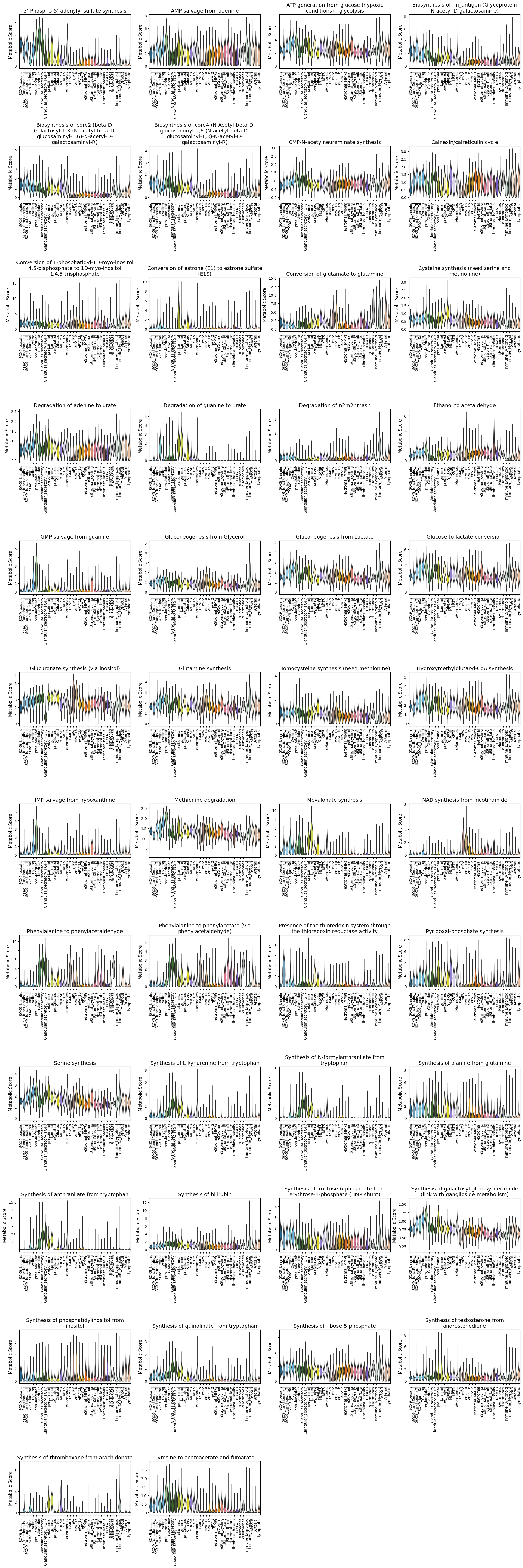
Violin plot

We can further inspect the metabolic score distribution across single cells per cell type for these markers:

fig, axes = sccellfie.plotting.create_multi_violin_plots(adata.metabolic_tasks,
                                                       features=both_markers,
                                                       groupby=cell_group,
                                                       stripplot=False,
                                                       n_cols=4,
                                                       ylabel='Metabolic Score'
                                                      )

Heatmap

As a summary visualization, we can create a heatmap of the identified metabolic task markers across cell types based on the aggregated scores into a cell-type level (found in agg calculated before):

filtered_agg = agg[both_markers]

filtered_agg.head()

Task	3'-Phospho-5'-adenylyl sulfate synthesis	AMP salvage from adenine	ATP generation from glucose (hypoxic conditions) - glycolysis	Biosynthesis of Tn_antigen (Glycoprotein N-acetyl-D-galactosamine)	Biosynthesis of core2 (beta-D-Galactosyl-1,3-(N-acetyl-beta-D-glucosaminyl-1,6)-N-acetyl-D-galactosaminyl-R)	Biosynthesis of core4 (N-Acetyl-beta-D-glucosaminyl-1,6-(N-acetyl-beta-D-glucosaminyl-1,3)-N-acetyl-D-galactosaminyl-R)	CMP-N-acetylneuraminate synthesis	Calnexin/calreticulin cycle	Conversion of 1-phosphatidyl-1D-myo-inositol 4,5-bisphosphate to 1D-myo-inositol 1,4,5-trisphosphate	Conversion of estrone (E1) to estrone sulfate (E1S)	...	Synthesis of anthranilate from tryptophan	Synthesis of bilirubin	Synthesis of fructose-6-phosphate from erythrose-4-phosphate (HMP shunt)	Synthesis of galactosyl glucosyl ceramide (link with ganglioside metabolism)	Synthesis of phosphatidylinositol from inositol	Synthesis of quinolinate from tryptophan	Synthesis of ribose-5-phosphate	Synthesis of testosterone from androstenedione	Synthesis of thromboxane from arachidonate	Tyrosine to acetoacetate and fumarate
Arterial	0.256560	1.675679	2.481569	0.683852	0.442055	0.344145	0.754417	0.773945	2.522644	0.104100	...	0.004131	0.796489	0.466867	0.699921	1.124336	0.031946	0.551582	1.033685	0.045549	0.030364
Ciliated	1.078283	1.451005	1.929947	1.445988	0.892795	0.846883	0.723723	0.565869	1.477182	1.089631	...	0.704579	1.092265	0.682542	0.758055	0.308139	0.291273	0.635575	0.865189	0.193303	0.553913
Cycling	2.098761	3.000086	3.718694	1.807871	1.074159	0.971235	1.017814	1.237260	1.803018	0.326987	...	0.273492	1.119333	1.211169	1.053797	0.542966	0.374733	0.957516	0.769935	0.106314	0.666761
Fibroblast_basalis	0.240646	1.469132	2.305450	0.710848	0.304962	0.355424	0.744974	0.695407	1.322372	0.140297	...	0.000000	0.951126	0.491220	0.580029	1.478609	0.081673	0.513473	1.045122	0.000000	0.026769
Glandular	3.829955	1.562031	2.227763	1.779426	1.111685	1.377226	0.908321	0.626390	1.595914	0.025143	...	2.093063	1.597565	0.794605	0.812703	0.527581	0.565066	0.695606	0.675938	0.201555	0.747315

5 rows × 46 columns

We then apply min-max normalization for better visualization:

normalized_markers = sccellfie.preprocessing.min_max_normalization(filtered_agg, axis=0)

Followed by the heatmap

# Create heatmap
plt.figure(figsize=(16, 9))
sns.heatmap(normalized_markers, cmap='YlOrBr', annot=False, linewidths=0.5,
            cbar_kws={'label': 'Min-max scaled metabolic score'})

plt.title('Metabolic Markers across Cell Types')
plt.ylabel('Cell Type')
plt.xlabel('Metabolic Task')
plt.tight_layout()