Spatial Overview
![]()
In this tutorial, we will use a processed 10X visium dataset of a Mouse Embryo (CytAssist FFPE). Coupled with H&E image, the visium section captures the transcriptome of a whole mouse embryo, enabling identification of regional metabolic processes across organs at early development.
This tutorial includes following steps:
Loading libraries
[1]:
import sccellfie

import scanpy as sc
import squidpy as sq

import pandas as pd
import numpy as np

import matplotlib.pyplot as plt

## To avoid warnings
import warnings
warnings.filterwarnings("ignore")
/home/jovyan/my-conda-envs/single_cell/lib/python3.10/site-packages/dask/dataframe/__init__.py:31: FutureWarning: The legacy Dask DataFrame implementation is deprecated and will be removed in a future version. Set the configuration option `dataframe.query-planning` to `True` or None to enable the new Dask Dataframe implementation and silence this warning.
  warnings.warn(
Define parameters
[2]:
SPOT_SIZE = 1.3
DPI = 150
ANNOTATION = 'leiden'
Loading data
The 10X Visium Cytassist dataset contains 6434 spots (n_obs) with 19288 genes (n_vars).
This is a processed dataset created by the OpenProblems community. Coupled with H&E image, the visium section captures the transcriptome of a whole mouse embryo, enabling identification of regional metabolic processes.
[3]:
adata = sc.read(filename='./data/MusMusculus_WholeEmbryo.h5ad',
                backup_url='https://zenodo.org/records/15330688/files/MusMusculus_WholeEmbryo.h5ad')
[4]:
sc.pl.spatial(adata,
              color=[None, 'total_counts'],
              size=SPOT_SIZE,
              cmap='YlGnBu',
              img_key="hires",
             )

Preprocessing spatial data
Gene names
Although gene names in the form of gene symbols are preferred, scCellFie supports the ENSEMBL IDs as used in .var_names of this AnnData object. scCellFie can internally convert ENSEMBL IDs into gene symbols. In this case the gene symbols can be found under the column name of feature_name.
[5]:
adata.var.head()
[5]:
| feature_id | feature_types | genome | n_cells_by_counts | mean_counts | log1p_mean_counts | pct_dropout_by_counts | total_counts | log1p_total_counts | n_cells | feature_name | |
|---|---|---|---|---|---|---|---|---|---|---|---|
| gene_ids | |||||||||||
| ENSMUSG00000051951 | ENSMUSG00000051951 | Gene Expression | mm10 | 742 | 0.147187 | 0.137313 | 88.467516 | 947.0 | 6.854354 | 742 | Xkr4 |
| ENSMUSG00000025900 | ENSMUSG00000025900 | Gene Expression | mm10 | 440 | 0.073205 | 0.070649 | 93.161330 | 471.0 | 6.156979 | 440 | Rp1 |
| ENSMUSG00000025902 | ENSMUSG00000025902 | Gene Expression | mm10 | 2614 | 0.852813 | 0.616705 | 59.372086 | 5487.0 | 8.610319 | 2614 | Sox17 |
| ENSMUSG00000025903 | ENSMUSG00000025903 | Gene Expression | mm10 | 5205 | 4.515853 | 1.707626 | 19.101647 | 29055.0 | 10.276980 | 5205 | Lypla1 |
| ENSMUSG00000033813 | ENSMUSG00000033813 | Gene Expression | mm10 | 5652 | 6.649984 | 2.034703 | 12.154181 | 42786.0 | 10.663990 | 5652 | Tcea1 |
(Optional) To work with gene symbols, we will replace the index names of adata.var with the column feature_name.
[6]:
adata.var.set_index('feature_name', inplace=True)
adata.var.head()
[6]:
| feature_id | feature_types | genome | n_cells_by_counts | mean_counts | log1p_mean_counts | pct_dropout_by_counts | total_counts | log1p_total_counts | n_cells | |
|---|---|---|---|---|---|---|---|---|---|---|
| feature_name | ||||||||||
| Xkr4 | ENSMUSG00000051951 | Gene Expression | mm10 | 742 | 0.147187 | 0.137313 | 88.467516 | 947.0 | 6.854354 | 742 |
| Rp1 | ENSMUSG00000025900 | Gene Expression | mm10 | 440 | 0.073205 | 0.070649 | 93.161330 | 471.0 | 6.156979 | 440 |
| Sox17 | ENSMUSG00000025902 | Gene Expression | mm10 | 2614 | 0.852813 | 0.616705 | 59.372086 | 5487.0 | 8.610319 | 2614 |
| Lypla1 | ENSMUSG00000025903 | Gene Expression | mm10 | 5205 | 4.515853 | 1.707626 | 19.101647 | 29055.0 | 10.276980 | 5205 |
| Tcea1 | ENSMUSG00000033813 | Gene Expression | mm10 | 5652 | 6.649984 | 2.034703 | 12.154181 | 42786.0 | 10.663990 | 5652 |
Raw counts
Raw counts are the inputs that scCellFie uses to internally perform all data processing that is needed.
We start preparing .X to contain the raw count matrix:
[7]:
adata.X = adata.layers['counts'].copy()
Run scCellFie
In current version, scCellFie supports human or mouse specific metabolic pathways. We will select organism='mouse' for the analysis.
[8]:
results = sccellfie.run_sccellfie_pipeline(adata,
                                           organism='mouse',
                                           sccellfie_data_folder=None,
                                           n_counts_col='total_counts',
                                           process_by_group=False,
                                           groupby=None,
                                           neighbors_key='neighbors',
                                           n_neighbors=10,
                                           batch_key=None,
                                           threshold_key='sccellfie_threshold',
                                           smooth_cells=True,
                                           alpha=0.33,
                                           chunk_size=5000,
                                           disable_pbar=False,
                                           save_folder=None,
                                           save_filename=None
                                          )
==== scCellFie Pipeline: Initializing ====
Loading scCellFie database for organism: mouse

==== scCellFie Pipeline: Processing entire dataset ====

---- scCellFie Step: Preprocessing data ----

---- scCellFie Step: Computing neighbors ----
2025-05-10 12:43:36.638794: E external/local_xla/xla/stream_executor/cuda/cuda_fft.cc:477] Unable to register cuFFT factory: Attempting to register factory for plugin cuFFT when one has already been registered
WARNING: All log messages before absl::InitializeLog() is called are written to STDERR
E0000 00:00:1746881016.659355   13629 cuda_dnn.cc:8310] Unable to register cuDNN factory: Attempting to register factory for plugin cuDNN when one has already been registered
E0000 00:00:1746881016.665681   13629 cuda_blas.cc:1418] Unable to register cuBLAS factory: Attempting to register factory for plugin cuBLAS when one has already been registered
2025-05-10 12:43:36.697329: I tensorflow/core/platform/cpu_feature_guard.cc:210] This TensorFlow binary is optimized to use available CPU instructions in performance-critical operations.
To enable the following instructions: AVX2 FMA, in other operations, rebuild TensorFlow with the appropriate compiler flags.
---- scCellFie Step: Preparing inputs ----
Gene names corrected to match database: 9
Shape of new adata object: (6434, 756)
Number of GPRs: 676
Shape of tasks by genes: (200, 756)
Shape of reactions by genes: (676, 756)
Shape of tasks by reactions: (200, 676)

---- scCellFie Step: Smoothing gene expression ----
Smoothing Expression: 100%|██████████| 1/1 [00:00<00:00, 1.15it/s]
---- scCellFie Step: Computing gene scores ----

---- scCellFie Step: Computing reaction activity ----
Cell Rxn Activities: 100%|██████████| 6434/6434 [00:53<00:00, 121.26it/s]
---- scCellFie Step: Computing metabolic task activity ----
Removed 1 metabolic tasks with zeros across all cells.

==== scCellFie Pipeline: Processing completed successfully ====
Export results
[9]:
results.keys()
[9]:
dict_keys(['adata', 'gpr_rules', 'task_by_gene', 'rxn_by_gene', 'task_by_rxn', 'rxn_info', 'task_info', 'thresholds', 'organism'])
To access metabolic activities, we need to inspect results['adata']:
The processed spatial data is located in the AnnData object
results['adata'].The reaction activities for each spot are located in the AnnData object
results['adata'].reactions.The metabolic task activities for each spot are located in the AnnData object
results['adata'].metabolic_tasks.
In particular:
results['adata']: contains gene expression in.X.results['adata'].layers['gene_scores']: contains gene scores as in the original CellFie paper.results['adata'].uns['Rxn-Max-Genes']: contains determinant genes for each reaction per spot.results['adata'].reactions: contains reaction scores in.Xso every scanpy function can be used on this object to visualize or compare values.results['adata'].metabolic_tasks: contains metabolic task scores in.Xso every scanpy function can be used on this object to visualize or compare values.
Other keys in the results dictionary are associated with the scCellFie database and are already filtered for the elements present in the dataset ('gpr_rules', 'task_by_gene', 'rxn_by_gene', 'task_by_rxn', 'rxn_info', 'task_info', 'thresholds', 'organism').
Save spatial results
We can save our spatial results contained in the AnnData objects (results['adata']) into a specific folder. Here we only need to specify the output folder, and the basename that our AnnData objects will have. This function below saves the expression object (results['adata']) and those containing scores for reactions and metabolic tasks (results['adata'].reactions and results['adata'].metabolic_tasks, respectively), as separate files.
[10]:
sccellfie.io.save_adata(adata=results['adata'], output_directory='./results', filename='Mouse_Spatial_scCellFie')
./results/Mouse_Spatial_scCellFie.h5ad was correctly saved
./results/Mouse_Spatial_scCellFie_reactions.h5ad was correctly saved
./results/Mouse_Spatial_scCellFie_metabolic_tasks.h5ad was correctly saved
Spatial visualization
scCellFie implements multiple visualizations, including plots to see metabolic activity across tissues.
In this case, we first define metabolic tasks that may be important for early stages of development:
[11]:
development = [
    'ATP generation from glucose (hypoxic conditions) - glycolysis',
    'Conversion of histidine to histamine',
    'O-linked glycosylation',
    'CMP-N-acetylneuraminate synthesis',
    'Conversion of estrone (E1) to estradiol-17beta (E2)',
    'Synthesis of inositol',
    'Conversion of 1-phosphatidyl-1D-myo-inositol 4,5-bisphosphate to 1D-myo-inositol 1,4,5-trisphosphate',
    'Synthesis of GABA',
    'Reactive oxygen species detoxification (H2O2 to H2O)',
    'S-adenosyl-L-methionine synthesis'
]
Then, we use a scCellFie plotting function to visualize them in space:
[12]:
fig, axes = sccellfie.plotting.plot_spatial(results['adata'].metabolic_tasks,
                                            keys=development ,
                                            img_key='hires',
                                            cmap='YlGnBu',
                                            size=SPOT_SIZE,
                                            use_raw=False,
                                            ncols=5,
                                            hspace=0.3,
                                            vmin=0
                                            )

Identification of metabolic markers
To identify markers, we can use different approaches. Here we show an approach based on TF-IDF, which comes from the Natural Language Processing field, and the logistic regression implemented in Scanpy.
Defining annotated regions for the selection of markers
To select markers, we need to define region annotations so the algorithms can focus on enriched activities in those regions.
As a demonstration, we will perform simple unsupervised clustering to define regional features of the whole embryo.
[13]:
sadata = adata.copy()
sc.pp.normalize_total(sadata, target_sum=1e4)
sc.pp.log1p(sadata)
sc.pp.highly_variable_genes(sadata, min_mean=0.0125, max_mean=3, min_disp=0.5)
sadata = sadata[:, sadata.var.highly_variable]
sc.tl.pca(sadata, svd_solver='arpack')
sc.pp.neighbors(sadata, n_neighbors=10, n_pcs=40)
sc.tl.umap(sadata)
sc.tl.leiden(sadata, resolution=0.4)
Then, we assign these annotations to our AnnData objects in under results['adata'] to help with further analyses and visualizations
[14]:
results['adata'].obs[ANNOTATION] = sadata.obs['leiden']
results['adata'].reactions.obs[ANNOTATION] = sadata.obs['leiden']
results['adata'].metabolic_tasks.obs[ANNOTATION] = sadata.obs['leiden']
[15]:
fig, axes = sccellfie.plotting.plot_spatial(results['adata'],
                                            keys=[None, ANNOTATION],
                                            img_key='hires',
                                            cmap='YlGnBu',
                                            size=SPOT_SIZE ,
                                            use_raw=False,
                                            ncols=2,
                                            dpi=DPI
                                            )

Marker detection using TF-IDF
scCellFie implements a TF-IDF (Term Frequency-Inverse Document Frequency) approach, adapted from the SoupX tool in R.
We define express_cut=5*np.log(2) to determine which spots are expressing each metabolic task. This value (5*np.log(2)) indicates that all reactions in the task are over the threshold value of the determinant gene (or “active”).
[16]:
mrks = sccellfie.external.quick_markers(results['adata'].metabolic_tasks,
                                        cluster_key=ANNOTATION,
                                        n_markers=20,
                                        express_cut=5*np.log(2))
[17]:
mrks.head()
[17]:
| gene | cluster | tf | idf | tf_idf | gene_frequency_outside_cluster | gene_frequency_global | second_best_tf | second_best_cluster | pval | qval | |
|---|---|---|---|---|---|---|---|---|---|---|---|
| 0 | Glycogen degradation | 0 | 0.905195 | 1.592333 | 1.441372 | 0.108051 | 0.203450 | 0.942529 | 15 | 0.0 | 0.0 |
| 1 | Hydroxymethylglutaryl-CoA synthesis | 0 | 0.802597 | 1.750950 | 1.405308 | 0.088100 | 0.173609 | 0.919540 | 15 | 0.0 | 0.0 |
| 2 | Acetoacetate synthesis | 0 | 0.709091 | 1.884865 | 1.336541 | 0.076095 | 0.151850 | 0.850575 | 15 | 0.0 | 0.0 |
| 3 | Synthesis of acetone | 0 | 0.709091 | 1.884865 | 1.336541 | 0.076095 | 0.151850 | 0.850575 | 15 | 0.0 | 0.0 |
| 4 | Synthesis of creatine from arginine | 0 | 0.990909 | 1.241558 | 1.230271 | 0.193503 | 0.288934 | 0.994253 | 15 | 0.0 | 0.0 |
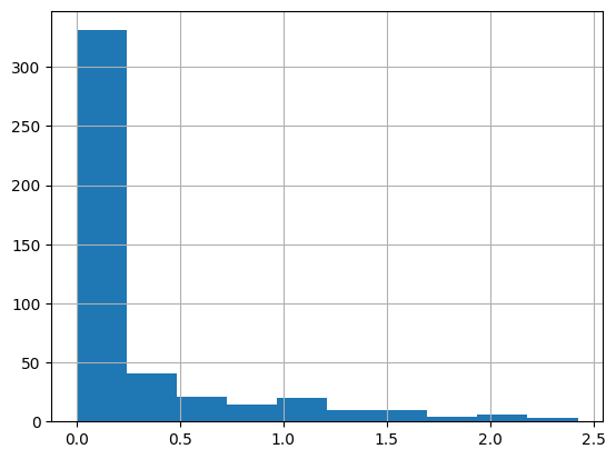
By examining the distributions of TF-IDF scores, we can filter the results to identify more specific tasks:
[18]:
mrks['tf_idf'].hist()
[18]:
<Axes: >
[19]:
# Scatter plot of TF vs IDF with TF-IDF as color
scatter = plt.scatter(mrks['tf'], mrks['idf'], c=mrks['tf_idf'], cmap='YlGnBu')
plt.colorbar(scatter)
plt.xlabel('TF')
plt.ylabel('IDF')
[19]:
Text(0, 0.5, 'IDF')
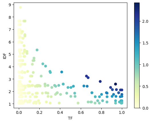
scCellFie includes a filtering function that fits a hyperbolic curve, while the user can define some thresholds based on the tf-idf scores, and the ratio between the top and second best clusters (tf_ratio).
[20]:
x_col = 'tf'
y_col = 'idf'
df = mrks
tfidf_threshold = 0.3
tf_ratio = 1.2

# Visualization
plt.figure(figsize=(6, 6))
# Plot all points
plt.scatter(df[x_col], df[y_col], alpha=0.5, c='lightgray', label='All points')
# Plot selected points
filtered_mrks, curve = sccellfie.external.filter_tfidf_markers(df, tf_col=x_col, idf_col=y_col,
                                                              tfidf_threshold=tfidf_threshold,
                                                              tf_ratio=tf_ratio)
plt.scatter(filtered_mrks[x_col], filtered_mrks[y_col], c='red', label='Selected points')
plt.plot(*curve, label='Fit curve')
plt.xlabel('TF')
plt.ylabel('IDF')
plt.legend()
[20]:
<matplotlib.legend.Legend at 0x7f5c746ef130>

A detailed list of the selected markers:
[21]:
filtered_mrks
[21]:
| gene | cluster | tf | idf | tf_idf | gene_frequency_outside_cluster | gene_frequency_global | second_best_tf | second_best_cluster | pval | qval | |
|---|---|---|---|---|---|---|---|---|---|---|---|
| 21 | Ethanol to acetaldehyde | 1 | 0.130841 | 4.184384 | 0.547490 | 0.004747 | 0.015232 | 0.058824 | 22 | 1.009938e-54 | 1.009938e-54 |
| 24 | UDP-galactose synthesis | 1 | 0.057944 | 5.214004 | 0.302120 | 0.000678 | 0.005440 | 0.057944 | 1 | 5.544113e-30 | 5.544113e-30 |
| 41 | Glycerol-3-phosphate synthesis | 2 | 0.107356 | 2.795542 | 0.300118 | 0.057157 | 0.061082 | 0.107356 | 2 | 2.263329e-05 | 0.000000e+00 |
| 62 | S-adenosyl-L-methionine synthesis | 3 | 0.301762 | 3.604566 | 1.087721 | 0.006355 | 0.027199 | 0.085324 | 11 | 5.039044e-130 | 5.039044e-130 |
| 63 | Homocysteine synthesis (need methionine) | 3 | 0.136564 | 4.478892 | 0.611655 | 0.001839 | 0.011346 | 0.037543 | 11 | 1.246696e-61 | 1.246696e-61 |
| 80 | Degradation of cytosine | 4 | 0.938497 | 2.583143 | 2.424271 | 0.012344 | 0.075536 | 0.430380 | 18 | 0.000000e+00 | 0.000000e+00 |
| 81 | Degradation of uracil | 4 | 0.938497 | 2.583143 | 2.424271 | 0.012344 | 0.075536 | 0.430380 | 18 | 0.000000e+00 | 0.000000e+00 |
| 100 | Glycerol-3-phosphate synthesis | 5 | 0.789731 | 2.795542 | 2.207726 | 0.011618 | 0.061082 | 0.107356 | 2 | 0.000000e+00 | 0.000000e+00 |
| 101 | Krebs cycle - NADH generation | 5 | 0.672372 | 3.099471 | 2.083996 | 0.002490 | 0.045073 | 0.031250 | 21 | 0.000000e+00 | 0.000000e+00 |
| 102 | Gluconeogenesis from Glycerol | 5 | 0.415648 | 3.559866 | 1.479651 | 0.002158 | 0.028443 | 0.025845 | 2 | 6.170726e-202 | 6.170726e-202 |
| 104 | Synthesis of fructose-6-phosphate from erythro... | 5 | 0.305623 | 3.522328 | 1.076506 | 0.010788 | 0.029531 | 0.139241 | 18 | 1.620833e-108 | 1.620833e-108 |
| 105 | Glycine synthesis | 5 | 0.259169 | 4.033153 | 1.045267 | 0.001328 | 0.017718 | 0.015905 | 2 | 3.962977e-122 | 3.962977e-122 |
| 106 | Heme synthesis | 5 | 0.232274 | 4.215475 | 0.979145 | 0.000000 | 0.014765 | 0.000000 | 22 | 2.854243e-119 | 2.854243e-119 |
| 109 | Methionine degradation | 5 | 0.146699 | 4.675007 | 0.685820 | 0.000000 | 0.009325 | 0.000000 | 22 | 2.170227e-74 | 2.170227e-74 |
| 110 | Serine synthesis | 5 | 0.146699 | 4.492686 | 0.659074 | 0.001992 | 0.011191 | 0.018809 | 7 | 1.714940e-61 | 1.714940e-61 |
| 120 | Conversion of histidine to histamine | 6 | 0.663043 | 2.409778 | 1.597787 | 0.055061 | 0.089835 | 0.529412 | 22 | 1.362200e-182 | 1.362200e-182 |
| 149 | Gluconeogenesis from Lactate | 7 | 0.216301 | 3.228088 | 0.698239 | 0.030417 | 0.039633 | 0.216301 | 7 | 7.201257e-34 | 1.629216e-44 |
| 160 | Synthesis of taurine from cysteine | 8 | 0.254839 | 2.430758 | 0.619451 | 0.079523 | 0.087970 | 0.254839 | 8 | 2.697996e-19 | 7.492150e-138 |
| 180 | Synthesis of taurine from cysteine | 9 | 0.631068 | 2.430758 | 1.533973 | 0.060571 | 0.087970 | 0.254839 | 8 | 7.492150e-138 | 7.492150e-138 |
| 200 | UDP-N-acetyl D-galactosamine synthesis | 10 | 0.078689 | 5.055780 | 0.397832 | 0.002774 | 0.006372 | 0.042071 | 9 | 4.986753e-22 | 4.986753e-22 |
| 220 | Synthesis of bilirubin | 11 | 0.986348 | 2.110058 | 2.081252 | 0.079954 | 0.121231 | 0.986348 | 11 | 4.338165e-281 | 0.000000e+00 |
| 221 | Conversion of asparate to asparagine | 11 | 0.907850 | 2.134718 | 1.938004 | 0.080606 | 0.118278 | 0.907850 | 11 | 7.658890e-231 | 0.000000e+00 |
| 222 | S-adenosyl-L-methionine synthesis | 11 | 0.085324 | 3.604566 | 0.307557 | 0.024426 | 0.027199 | 0.085324 | 11 | 2.733811e-07 | 5.039044e-130 |
| 306 | (R)-3-Hydroxybutanoate synthesis | 15 | 0.505747 | 2.311013 | 1.168788 | 0.087859 | 0.099161 | 0.505747 | 15 | 9.802464e-44 | 3.015513e-201 |
| 342 | Conversion of estrone (E1) to estradiol-17beta... | 17 | 0.057971 | 6.572127 | 0.380993 | 0.000159 | 0.001399 | 0.003226 | 8 | 3.233538e-13 | 3.233538e-13 |
| 343 | Synthesis of testosterone from androstenedione | 17 | 0.057971 | 6.466767 | 0.374885 | 0.000318 | 0.001554 | 0.057971 | 17 | 1.587698e-12 | 1.587698e-12 |
| 360 | Degradation of cytosine | 18 | 0.430380 | 2.583143 | 1.111732 | 0.071125 | 0.075536 | 0.430380 | 18 | 2.476438e-18 | 0.000000e+00 |
| 361 | Degradation of uracil | 18 | 0.430380 | 2.583143 | 1.111732 | 0.071125 | 0.075536 | 0.430380 | 18 | 2.476438e-18 | 0.000000e+00 |
| 363 | Synthesis of fructose-6-phosphate from erythro... | 18 | 0.139241 | 3.522328 | 0.490451 | 0.028167 | 0.029531 | 0.139241 | 18 | 1.745384e-05 | 1.620833e-108 |
| 380 | Conversion of 1-phosphatidyl-1D-myo-inositol 4... | 19 | 0.346667 | 2.477783 | 0.858965 | 0.080830 | 0.083929 | 0.346667 | 19 | 1.178491e-10 | 2.657205e-96 |
| 420 | Gluconeogenesis from Lactate | 21 | 0.656250 | 3.228088 | 2.118433 | 0.033438 | 0.039633 | 0.216301 | 7 | 1.629216e-44 | 1.629216e-44 |
| 421 | (R)-3-Hydroxybutanoate synthesis | 21 | 0.890625 | 2.311013 | 2.058246 | 0.091209 | 0.099161 | 0.505747 | 15 | 1.938126e-50 | 3.015513e-201 |
| 430 | Gluconeogenesis from pyruvate | 21 | 0.078125 | 5.214004 | 0.407344 | 0.004710 | 0.005440 | 0.053292 | 7 | 2.143704e-05 | 8.758385e-14 |
| 431 | UDP-glucose synthesis | 21 | 0.046875 | 7.670739 | 0.359566 | 0.000000 | 0.000466 | 0.000000 | 22 | 9.390129e-07 | 9.390129e-07 |
| 440 | Conversion of histidine to histamine | 22 | 0.529412 | 2.409778 | 1.275765 | 0.088671 | 0.089835 | 0.529412 | 22 | 4.510992e-06 | 1.362200e-182 |
| 441 | Synthesis of phosphatidylinositol from inositol | 22 | 0.176471 | 5.335365 | 0.941535 | 0.004363 | 0.004818 | 0.055000 | 14 | 6.580741e-05 | 9.784487e-10 |
| 442 | Conversion of glycine to pyruvate | 22 | 0.058824 | 7.670739 | 0.451220 | 0.000312 | 0.000466 | 0.003976 | 2 | 7.906940e-03 | 7.906940e-03 |
Finally, we will get the unique list of filtered markers
[22]:
tf_idf_mrks = filtered_mrks['gene'].unique().tolist()
len(tf_idf_mrks)
[22]:
28
[23]:
tf_idf_mrks
[23]:
['Ethanol to acetaldehyde',
 'UDP-galactose synthesis',
 'Glycerol-3-phosphate synthesis',
 'S-adenosyl-L-methionine synthesis',
 'Homocysteine synthesis (need methionine)',
 'Degradation of cytosine',
 'Degradation of uracil',
 'Krebs cycle - NADH generation',
 'Gluconeogenesis from Glycerol',
 'Synthesis of fructose-6-phosphate from erythrose-4-phosphate (HMP shunt)',
 'Glycine synthesis',
 'Heme synthesis',
 'Methionine degradation',
 'Serine synthesis',
 'Conversion of histidine to histamine',
 'Gluconeogenesis from Lactate',
 'Synthesis of taurine from cysteine',
 'UDP-N-acetyl D-galactosamine synthesis',
 'Synthesis of bilirubin',
 'Conversion of asparate to asparagine',
 '(R)-3-Hydroxybutanoate synthesis',
 'Conversion of estrone (E1) to estradiol-17beta (E2)',
 'Synthesis of testosterone from androstenedione',
 'Conversion of 1-phosphatidyl-1D-myo-inositol 4,5-bisphosphate to 1D-myo-inositol 1,4,5-trisphosphate',
 'Gluconeogenesis from pyruvate',
 'UDP-glucose synthesis',
 'Synthesis of phosphatidylinositol from inositol',
 'Conversion of glycine to pyruvate']
Detection using Logistic Regression in Scanpy
We can also use logistic regression, as implemented in Scanpy, to identify metabolic task markers:
[24]:
method = 'logreg'
sc.tl.rank_genes_groups(results['adata'].metabolic_tasks, groupby=ANNOTATION, method=method,
                       use_raw=False, key_added=method)
sc.pl.rank_genes_groups(results['adata'].metabolic_tasks, n_genes=20, sharey=True, key=method, fontsize=4)

Extract the result in a dataframe
[25]:
scanpy_df = sc.get.rank_genes_groups_df(results['adata'].metabolic_tasks,
                                        key=method,
                                        group=None)

scanpy_df.head()
[25]:
| group | names | scores | |
|---|---|---|---|
| 0 | 0 | Mannose degradation (to fructose-6-phosphate) | 1.480771 |
| 1 | 0 | Degradation of cytosine | 1.127286 |
| 2 | 0 | Degradation of uracil | 1.127286 |
| 3 | 0 | Degradation of adenine to urate | 0.926927 |
| 4 | 0 | ATP generation from glucose (hypoxic condition... | 0.905349 |
We can filter the logistic regression markers based on their scores:
[26]:
scanpy_df['scores'].hist()
[26]:
<Axes: >

[27]:
# Filter based on score threshold
scores_threshold = 1.5
filtered_scanpy_mrks = scanpy_df.loc[scanpy_df['scores'] > scores_threshold]
[28]:
filtered_scanpy_mrks
[28]:
| group | names | scores | |
|---|---|---|---|
| 597 | 3 | Conversion of asparate to asparagine | 1.626031 |
| 796 | 4 | Degradation of uracil | 1.820949 |
| 797 | 4 | Degradation of cytosine | 1.820949 |
| 798 | 4 | Presence of the thioredoxin system through the... | 1.747238 |
| 995 | 5 | Oxidative phosphorylation via succinate-coenzy... | 1.639906 |
| 1194 | 6 | Conversion of histidine to histamine | 1.805179 |
| 1393 | 7 | Conversion of histidine to histamine | 1.569943 |
| 1791 | 9 | Synthesis of taurine from cysteine | 1.565231 |
| 1990 | 10 | UDP-N-acetyl D-galactosamine synthesis | 1.535176 |
| 2189 | 11 | Synthesis of bilirubin | 1.540485 |
| 2388 | 12 | Synthesis of creatine from arginine | 1.737556 |
| 2587 | 13 | Synthesis of creatine from arginine | 1.926244 |
| 2786 | 14 | Fucosylation (addition of fucose) | 1.906202 |
| 2787 | 14 | Conversion of estrone (E1) to estrone sulfate ... | 1.570353 |
| 2985 | 15 | Synthesis of creatine from arginine | 2.710084 |
| 2986 | 15 | Conversion of estrone (E1) to estrone sulfate ... | 1.896867 |
| 3383 | 17 | Synthesis of fructose-6-phosphate from erythro... | 1.597093 |
| 3582 | 18 | Glutathionate synthesis | 1.662967 |
| 3980 | 20 | NAD synthesis from nicotinamide | 1.608922 |
| 4179 | 21 | Glycogen degradation | 2.259699 |
| 4180 | 21 | Oxidative phosphorylation via succinate-coenzy... | 1.691183 |
[29]:
# Convert them to a list
scanpy_mrks = filtered_scanpy_mrks['names'].unique().tolist()
len(scanpy_mrks)
[29]:
16
Combining TF-IDF & Logistic Regression Markers
We can combine the metabolic tasks from different approaches:
[32]:
both_markers = sorted(set(tf_idf_mrks).union(set(scanpy_mrks)))
len(both_markers)
[32]:
36
Select only highly active markers
We can filter the markers based on their activity level by aggregating the metabolic activity to the cell-type level. Here, we consider only metabolic tasks with a prudent score at the cluster level (> 1)
[33]:
agg = sccellfie.expression.aggregation.agg_expression_cells(results['adata'].metabolic_tasks[:, both_markers],
                                                            ANNOTATION,
                                                            agg_func='trimean')
agg = agg.T.loc[(agg.T > 1.).any(axis=1)]

both_markers = agg.index.tolist()
Then we can visualize them in space:
[34]:
## visualise only 5 markers due to notebook size
fig, axes = sccellfie.plotting.plot_spatial(results['adata'].metabolic_tasks,
                                            keys=[ANNOTATION] + both_markers[0:5],
                                            img_key='hires',
                                            cmap='YlGnBu',
                                            size=SPOT_SIZE,
                                            use_raw=False,
                                            ncols=3,
                                            vmin=0
                                            )

Spatial patterns
scCellFie supports multiple algorithms to identify patterns across space, including the analysis of hotspots, assortativity, and autocorrelation (Moran’s I).
To illustrate the identification of spatial patterns, in this tutorial we will use the autocorrelation approach.
Generate spatial knn network
Methods to identify spatial patterns often rely on spatial neighbors, so we start computing our KNN network based on spatial locations. We compute this network in our original AnnData object and the one containing the metabolic scores for each task, in this case based on the 10-nearest neighbors:
[35]:
sccellfie.spatial.create_knn_network(adata, n_neighbors=10, spatial_key='spatial')
[36]:
sccellfie.spatial.create_knn_network(results['adata'].metabolic_tasks, n_neighbors=10, spatial_key='spatial')
Computing autocorrelation (Moran’s I coefficient)
Moran’s I is a measure of spatial autocorrelation, which quantifies how similar a variable is to itself in nearby spatial locations. In the context of spatial transcriptomics, where each spot or cell has a spatial coordinate and, here, an inferred metabolic activity score, Moran’s I can identify whether these scores are spatially clustered (positive autocorrelation), dispersed (negative autocorrelation), or randomly distributed (no autocorrelation).
Let:
\((x_i)\) be the metabolic activity score at spatial location (\(i\)),
\((\bar{x})\) be the mean metabolic activity across all locations,
\(( w_{ij} )\) be the spatial weight between location (\(i\)) and (\(j\)) (e.g., inverse distance or adjacency),
\((N)\) be the total number of spatial locations.
Then Moran’s I is computed as:
where:
Interpretation:
( I > 0 ): Positive spatial autocorrelation (similar metabolic activities cluster spatially).
( I < 0 ): Negative spatial autocorrelation (dissimilar metabolic activities are near each other).
( I \(\approx\) 0 ): No spatial autocorrelation (random spatial distribution).
[37]:
sq.gr.spatial_autocorr(
    results['adata'].metabolic_tasks,
    mode="moran",
    n_perms=1000,
    n_jobs=1,
)
[38]:
moran = results['adata'].metabolic_tasks.uns['moranI']
[39]:
moran
[39]:
| I | pval_norm | var_norm | pval_z_sim | pval_sim | var_sim | pval_norm_fdr_bh | pval_z_sim_fdr_bh | pval_sim_fdr_bh | |
|---|---|---|---|---|---|---|---|---|---|
| Heme synthesis | 0.943502 | 0.0 | 0.000057 | 0.0 | 0.000999 | 0.000154 | 0.0 | 0.0 | 0.000999 |
| Tyrosine to acetoacetate and fumarate | 0.931207 | 0.0 | 0.000057 | 0.0 | 0.000999 | 0.000147 | 0.0 | 0.0 | 0.000999 |
| Synthesis of bilirubin | 0.918218 | 0.0 | 0.000057 | 0.0 | 0.000999 | 0.000150 | 0.0 | 0.0 | 0.000999 |
| Synthesis of globoside (link with globoside metabolism) | 0.912165 | 0.0 | 0.000057 | 0.0 | 0.000999 | 0.000147 | 0.0 | 0.0 | 0.000999 |
| Synthesis of glucocerebroside | 0.908566 | 0.0 | 0.000057 | 0.0 | 0.000999 | 0.000147 | 0.0 | 0.0 | 0.000999 |
| ... | ... | ... | ... | ... | ... | ... | ... | ... | ... |
| Synthesis of anthranilate from tryptophan | 0.243993 | 0.0 | 0.000057 | 0.0 | 0.000999 | 0.000063 | 0.0 | 0.0 | 0.000999 |
| Synthesis of L-kynurenine from tryptophan | 0.177245 | 0.0 | 0.000057 | 0.0 | 0.000999 | 0.000054 | 0.0 | 0.0 | 0.000999 |
| GDP-L-fucose synthesis | 0.165651 | 0.0 | 0.000057 | 0.0 | 0.000999 | 0.000044 | 0.0 | 0.0 | 0.000999 |
| Phosphatidyl-inositol to glucosaminyl-acylphosphatidylinositol | 0.155917 | 0.0 | 0.000057 | 0.0 | 0.000999 | 0.000046 | 0.0 | 0.0 | 0.000999 |
| Conversion of glutamate to glutamine | 0.136900 | 0.0 | 0.000057 | 0.0 | 0.000999 | 0.000046 | 0.0 | 0.0 | 0.000999 |
199 rows × 9 columns
Visualize spatially informative variables (High Moran’s I coefficient)
[40]:
moran['I'].hist()
[40]:
<Axes: >

We can set a threshold to select highly autocorrelated featurres, in this case we use a Moran’s I of at least 0.6
[47]:
coef_threshold = 0.6
[48]:
top_moran = moran[moran['I'].abs() >= coef_threshold].dropna().sort_values(by='I', ascending=False)
[49]:
top_moran
[49]:
| I | pval_norm | var_norm | pval_z_sim | pval_sim | var_sim | pval_norm_fdr_bh | pval_z_sim_fdr_bh | pval_sim_fdr_bh | |
|---|---|---|---|---|---|---|---|---|---|
| Heme synthesis | 0.943502 | 0.0 | 0.000057 | 0.0 | 0.000999 | 0.000154 | 0.0 | 0.0 | 0.000999 |
| Tyrosine to acetoacetate and fumarate | 0.931207 | 0.0 | 0.000057 | 0.0 | 0.000999 | 0.000147 | 0.0 | 0.0 | 0.000999 |
| Synthesis of bilirubin | 0.918218 | 0.0 | 0.000057 | 0.0 | 0.000999 | 0.000150 | 0.0 | 0.0 | 0.000999 |
| Synthesis of globoside (link with globoside metabolism) | 0.912165 | 0.0 | 0.000057 | 0.0 | 0.000999 | 0.000147 | 0.0 | 0.0 | 0.000999 |
| Synthesis of glucocerebroside | 0.908566 | 0.0 | 0.000057 | 0.0 | 0.000999 | 0.000147 | 0.0 | 0.0 | 0.000999 |
| ... | ... | ... | ... | ... | ... | ... | ... | ... | ... |
| Inosine monophosphate synthesis (IMP) | 0.609340 | 0.0 | 0.000057 | 0.0 | 0.000999 | 0.000090 | 0.0 | 0.0 | 0.000999 |
| Degradation of n2m2nmasn | 0.608268 | 0.0 | 0.000057 | 0.0 | 0.000999 | 0.000101 | 0.0 | 0.0 | 0.000999 |
| N-glycan processing (ER) | 0.604972 | 0.0 | 0.000057 | 0.0 | 0.000999 | 0.000089 | 0.0 | 0.0 | 0.000999 |
| Deoxyadenosine triphosphate synthesis (dATP) | 0.604090 | 0.0 | 0.000057 | 0.0 | 0.000999 | 0.000090 | 0.0 | 0.0 | 0.000999 |
| Deoxycytidine triphosphate synthesis (dCTP) | 0.600372 | 0.0 | 0.000057 | 0.0 | 0.000999 | 0.000099 | 0.0 | 0.0 | 0.000999 |
145 rows × 9 columns
[50]:
spa_informative_var = list(top_moran.index)
Then, we can further filter top metabolic tasks to pick those with a high activity in at least one Visium spot
[51]:
mt_df = results['adata'].metabolic_tasks.to_df().max(axis=0)
spa_informative_var = list(mt_df[spa_informative_var][mt_df[spa_informative_var] > 5*np.log(2)].index)
[52]:
spa_informative_var
[52]:
['Heme synthesis',
 'Synthesis of bilirubin',
 'Homocysteine degradation',
 'Krebs cycle - NADH generation',
 'Degradation of uracil',
 'Degradation of cytosine',
 'Methionine degradation',
 'Cysteine synthesis (need serine and methionine)',
 'Gluconeogenesis from Glycerol',
 'Glycerol-3-phosphate synthesis',
 'Oxidative phosphorylation via succinate-coenzyme Q oxidoreductase (COMPLEX II)',
 'Gluconeogenesis from pyruvate',
 'Phenylalanine to tyrosine',
 'Gluconeogenesis from Lactate',
 'Synthesis of GABA',
 'Glutathionate synthesis',
 'Reactive oxygen species detoxification (H2O2 to H2O)',
 'Synthesis of creatine from arginine',
 'Synthesis of malonyl-coa',
 'Synthesis of acetone',
 'Acetoacetate synthesis',
 'ATP generation from glucose (hypoxic conditions) - glycolysis',
 'Hydroxymethylglutaryl-CoA synthesis',
 'Glycogen degradation',
 'Glycine synthesis',
 'Conversion of asparate to asparagine',
 'Homocysteine synthesis (need methionine)',
 'Synthesis of methylglyoxal',
 '(R)-3-Hydroxybutanoate synthesis',
 'Serine synthesis',
 'UDP-glucose synthesis',
 'Synthesis of fructose-6-phosphate from erythrose-4-phosphate (HMP shunt)',
 'Glucuronate synthesis (via udp-glucose)',
 'UDP-glucuronate synthesis',
 'S-adenosyl-L-methionine synthesis',
 "3'-Phospho-5'-adenylyl sulfate synthesis",
 'Conversion of histidine to histamine',
 'Mannose trimming (mannosidase)',
 'Synthesis of inositol',
 'UDP-N-acetyl D-galactosamine synthesis',
 'Conversion of glycine to pyruvate',
 'Presence of the thioredoxin system through the thioredoxin reductase activity',
 'Biosynthesis of m4mpdol_U',
 'Conversion of 1-phosphatidyl-1D-myo-inositol 4,5-bisphosphate to 1D-myo-inositol 1,4,5-trisphosphate',
 'Synthesis of ornithine from glutamine',
 'Conversion of estrone (E1) to estrone sulfate (E1S)',
 'Conversion of glutamate to proline',
 'CMP-N-acetylneuraminate synthesis',
 'Synthesis of taurine from cysteine']
Finally, we can visualize them in space to observe the patterns they have:
[53]:
spa_inf_titles = [t + " (Moran's I: {:.3f})".format(top_moran.loc[t, 'I']) for t in spa_informative_var ]

## visualise only 5 markers due to notebook size
fig, axes = sccellfie.plotting.plot_spatial(results['adata'].metabolic_tasks,
                                            keys=spa_informative_var [0:5],
                                            img_key='hires',
                                            cmap='YlGnBu',
                                            size=SPOT_SIZE,
                                            use_raw=False,
                                            ncols=3,
                                            vmin=0,
                                            hspace=0.2,
                                            title=spa_inf_titles
                                            )

Cell-cell communication
For spatial data, scCellFie can predict cell-cell communication (CCC) by calculating the co-localization of the synthesis of a metabolite and the receptor expression within a pre-defined neighborhood. This is different to the approach we take in single-cell data as shown in this tutorial, where we infer CCC by first aggregating metabolic scores and gene expression into a cell type level, and then using them to compute a communication score.
Defining neighborhoods
We start defining our neighborhoods by finding an acceptable ratio where each spot is allocated with its immediate neighbors:
[54]:
r = sccellfie.spatial.compute_neighbor_distribution(
    adata,
    radius_range=(100, 1500),  # adjust based on your data's scale
    n_points=200,
    spatial_key='spatial'
)
[55]:
sccellfie.plotting.spatial.plot_neighbor_distribution(r)
[55]:
(<Figure size 1500x800 with 4 Axes>, GridSpec(2, 3))

Here, we select a radius of 450 to keep mode of neighbors (in distribution) of ~6 (immediate neighbors).
[56]:
radius = 450
Data preparation
scCellFie generates separate AnnData objects containing either reaction scores (adata.reactions) or task scores (adata.metabolic_tasks). Therefore, to infer cell-cell communication, we need to put metabolic task scores together with gene expression in the same AnnData object.
Here, our adata already contains log1p(CP10k) values, as scCellFie processed it when running its pipeline.
Then, we transfer metabolic scores into the AnnData object containing gene expression. For this, we use a built-in function in scCellFie to transfer features from one source adata into another target adata. In this case we transfer all metabolic tasks (by using var_names=adata.metabolic_tasks.var_names).
[57]:
adata_updated = sccellfie.preprocessing.adata_utils.transfer_variables(
    adata_target=adata,
    adata_source=results['adata'].metabolic_tasks,
    var_names=results['adata'].metabolic_tasks.var_names
)

adata_updated
[57]:
AnnData object with n_obs × n_vars = 6434 × 19487
    obs: 'in_tissue', 'array_row', 'array_col', 'n_genes_by_counts', 'log1p_n_genes_by_counts', 'total_counts', 'log1p_total_counts', 'pct_counts_in_top_50_genes', 'pct_counts_in_top_100_genes', 'pct_counts_in_top_200_genes', 'pct_counts_in_top_500_genes', 'n_genes', 'size_factors'
    uns: 'dataset_description', 'dataset_id', 'dataset_name', 'dataset_organism', 'dataset_reference', 'dataset_summary', 'dataset_url', 'normalization_id', 'spatial', 'normalization', 'neighbors', 'umap', 'spatial_neighbors', 'spatial_network'
    obsm: 'spatial', 'X_pca', 'X_umap'
    layers: 'counts', 'normalized'
    obsp: 'distances', 'connectivities', 'spatial_connectivities', 'spatial_distances'
Compute cell-cell communication based on synthesis and receptor pairs
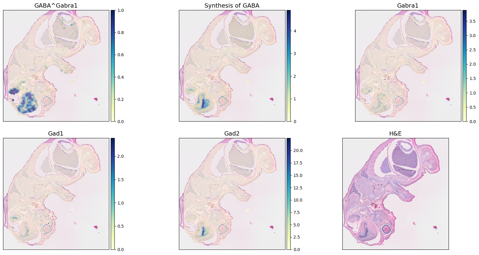
As a demonstration, we selected the 'Synthesis of GABA' to compute local co-localization scores for the pathway and its represented receptor Gabra1.
A 'pairwise_concordance' score is computed by first identifying neighboring spots within a predefined radius (already done a couple of steps above). Each sender-receiver spot pair within the neighborhood is then evaluated.
To measure co-localization, we account for pairs of spots where one partner presents a metabolic score above a threshold and the other has the receptor expression above another threshold. Here, we do not input any threshold value to the function, so scCellFie set them by default to be mean metabolic score and receptor expression across all spots. Finally, the co-localization score corresponds to the fraction between the pairs of spots that are above the respective thresholds and the total number of pairs within a given neighborhood.
[58]:
adata_updated.obs['GABA^Gabra1'] = sccellfie.communication.compute_local_colocalization_scores(
    adata_updated,
    var1='Synthesis of GABA',
    var2='Gabra1',
    neighbors_radius=radius,
    method='pairwise_concordance',
    min_neighbors=3,
    spatial_key='spatial',
    inplace=False
)
Then, we can visualize these synthesis of GABA, the expression of the receptor, the co-localization communication scores, and the main enzymes involved in this synthesis (Gad1 and Gad2)
[59]:
fig, axes = sccellfie.plotting.plot_spatial(adata_updated,
                                            keys=['GABA^Gabra1',
                                                  'Synthesis of GABA',
                                                  'Gabra1', # Receptor
                                                  'Gad1', # Synthase
                                                  'Gad2', # Synthase,
                                                  None # H&E
                                                  ],
                                            img_key="hires",
                                            cmap='YlGnBu',
                                            size=SPOT_SIZE,
                                            use_raw=False,
                                            ncols=3,
                                            vmin=0,
                                            hspace=0.15
                                            )