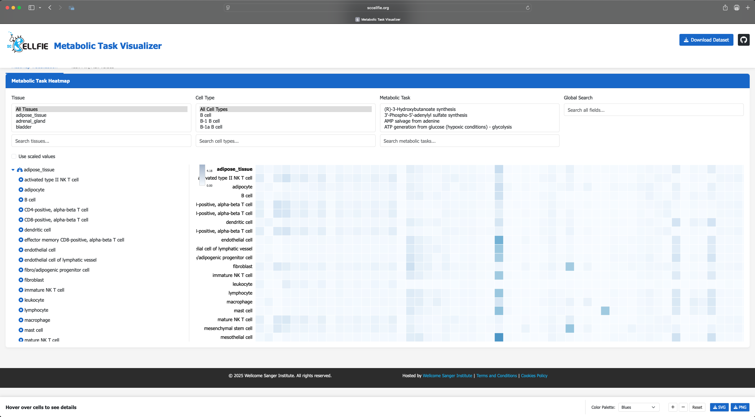
Metabolic Task Visualizer

In this tutorial, we will walk you through how to export scCellFie’s inferred metabolic activities to be visualized in the scCellFie Metabolic Task Visualizer.

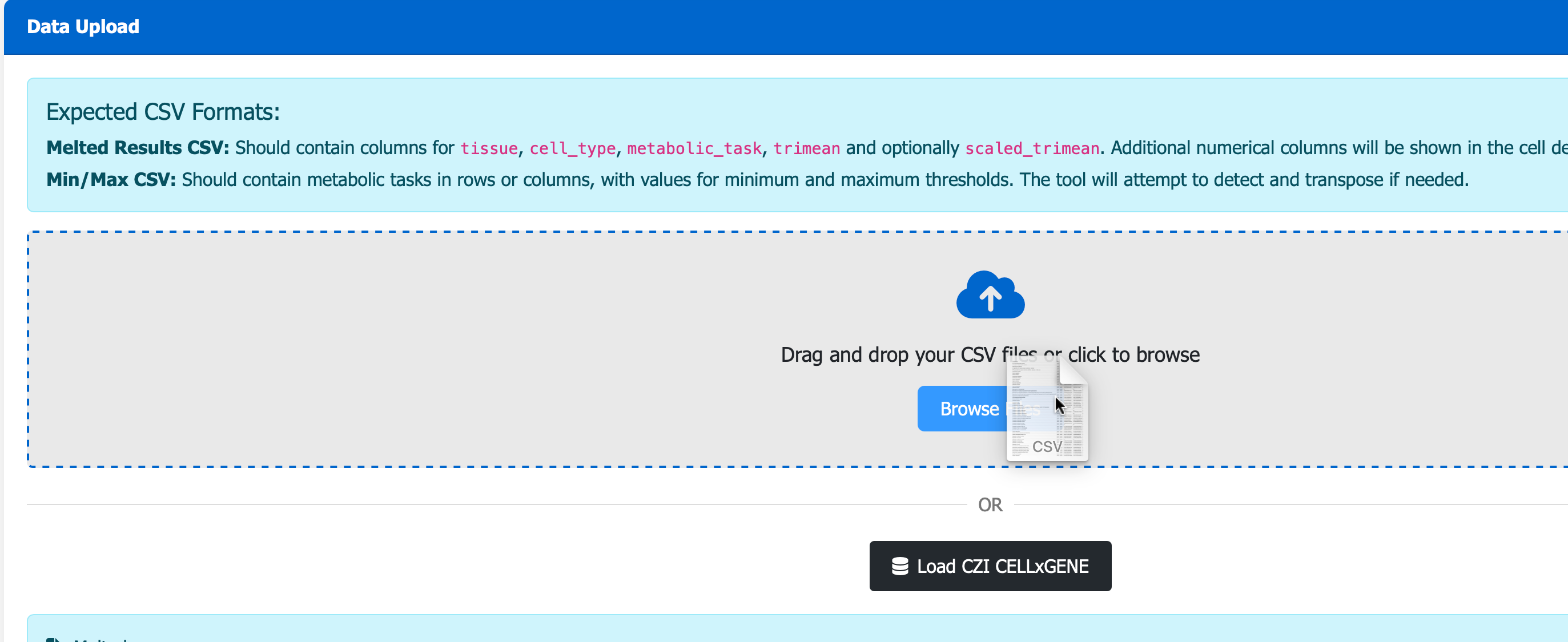
The visualizer enables users to drag and drop the .csv output to visualize results interactively through the portal.

The dataset we are using is a downsampled version of the Human Endometrial Cell Atlas found in The Repoductive Cell Atlas (Mareckova & Garcia-Alonso et al 2023).

This tutorial includes following steps:

• Loading libraries

• Loading endometrium data

• Run scCellFie

• Export results

• Online visualizations

• Additional local visualizations

Loading libraries

import sccellfie
import scanpy as sc
import pandas as pd
import numpy as np

import matplotlib.pyplot as plt
import seaborn as sns
import glasbey

## To avoid warnings
import warnings
warnings.filterwarnings("ignore")

First, let’s define file paths for all results of our analysis

results_dir = './results/endometrium2023/'

Loading endometrium data

The downsampled Human Endometrial Cell Atlas contains ~90k cells (n_obs) with 17,736 genes (n_vars).

This is a processed data, with raw count matrix stored in .X, including 36 cell type annotations in .obs['celltype'].

adata = sc.read(filename='./data/HECA-Subset.h5ad',
                backup_url='https://zenodo.org/records/15072628/files/HECA-Subset.h5ad')

adata

AnnData object with n_obs × n_vars = 90001 × 17736
    obs: 'n_genes', 'sample', 'percent_mito', 'n_counts', 'Endometriosis_stage', 'Endometriosis', 'Hormonal treatment', 'Binary Stage', 'Stage', 'phase', 'dataset', 'Age', 'lineage', 'celltype', 'label_long'
    var: 'gene_ids', 'feature_types'
    uns: 'Binary Stage_colors', 'Biopsy_type_colors', 'Endometrial_pathology_colors', 'Endometriosis_stage_colors', 'GarciaAlonso_celltype_colors', 'Group_colors', 'Hormonal treatment_colors', 'Library_genotype_colors', 'Mareckova_celltype_colors', 'Mareckova_epi_celltype_colors', 'Mareckova_lineage_colors', 'Processing_colors', 'Symbol_colors', 'Tan_cellsubtypes_colors', 'Tan_celltype_colors', 'Treatment_colors', 'celltype_colors', 'dataset_colors', 'genotype_colors', 'hvg', 'label_long_colors', 'leiden', 'leiden_R_colors', 'leiden_colors', 'lineage_colors', 'neighbors', 'phase_colors', 'umap'
    obsm: 'X_scVI', 'X_umap'
    obsp: 'connectivities', 'distances'

adata.uns['neighbors']

{'connectivities_key': 'connectivities',
 'distances_key': 'distances',
 'params': {'method': 'umap',
  'metric': 'euclidean',
  'n_neighbors': 15,
  'random_state': 0,
  'use_rep': 'X_scVI'}}

However, we need the raw counts of all genes. So we load the raw version of it and transfer annotations from the processed dataset.

Run scCellFie

Now we run scCellFie on the raw data.

scCellFie provides an option to compute n_neighbors. Since the this dataset contains a pre-computed .uns['neighbors'], we will use neighbors_key='neighbors' instead.

Users may also want to tweak the parameter chunk_size for computing large datasets on local machines.

results = sccellfie.run_sccellfie_pipeline(adata,
                                           organism='human',
                                           sccellfie_data_folder=None,
                                           n_counts_col='n_counts',
                                           process_by_group=False,
                                           groupby=None,
                                           neighbors_key='neighbors',
                                           batch_key=None,  # Specify batch_key or leave as None
                                           threshold_key='sccellfie_threshold',
                                           smooth_cells=True,
                                           alpha=0.33,
                                           chunk_size=5000,
                                           disable_pbar=False,
                                           save_folder=None,
                                           save_filename=None
                                          )

==== scCellFie Pipeline: Initializing ====
Loading scCellFie database for organism: human

==== scCellFie Pipeline: Processing entire dataset ====

---- scCellFie Step: Preprocessing data ----

---- scCellFie Step: Preparing inputs ----
Gene names corrected to match database: 22
Shape of new adata object: (90001, 839)
Number of GPRs: 748
Shape of tasks by genes: (215, 839)
Shape of reactions by genes: (748, 839)
Shape of tasks by reactions: (215, 748)

---- scCellFie Step: Smoothing gene expression ----

Smoothing Expression: 100%|██████████| 19/19 [00:44<00:00,  2.33s/it]

---- scCellFie Step: Computing gene scores ----

---- scCellFie Step: Computing reaction activity ----

Cell Rxn Activities: 100%|██████████| 90001/90001 [07:51<00:00, 190.95it/s]

---- scCellFie Step: Computing metabolic task activity ----
Removed 0 metabolic tasks with zeros across all cells.

==== scCellFie Pipeline: Processing completed successfully ====

Export results

The scCellFie results are stored as dictionary and can be retrieved by the dictionary keys.

results.keys()

dict_keys(['adata', 'gpr_rules', 'task_by_gene', 'rxn_by_gene', 'task_by_rxn', 'rxn_info', 'task_info', 'thresholds', 'organism'])

To access metabolic activities, we need to inspect results['adata']:

• The processed single-cell data is located in the AnnData object results['adata'].

• The reaction activities for each cell are located in the AnnData object results['adata'].reactions.

• The metabolic task activities for each cell are located in the AnnData object results['adata'].metabolic_tasks.

In particular:

• results['adata']: contains gene expression in .X.

• results['adata'].layers['gene_scores']: contains gene scores as in the original CellFie paper.

• results['adata'].uns['Rxn-Max-Genes']: contains determinant genes for each reaction per cell.

• results['adata'].reactions: contains reaction scores in .X so every scanpy function can be used on this object to visualize or compare values.

• results['adata'].metabolic_tasks: contains metabolic task scores in .X so every scanpy function can be used on this object to visualize or compare values.

Other keys in the results dictionary are associated with the scCellFie database and are already filtered for the elements present in the dataset ('gpr_rules', 'task_by_gene', 'rxn_by_gene', 'task_by_rxn', 'rxn_info', 'task_info', 'thresholds', 'organism').

Summarise results into a table to use on scCellFie Metabolic Task Visualizer

We want metabolic scores at a cell type level. Here, the column summarizing these groups is 'celltype'.

cell_group = 'celltype'

report = sccellfie.reports.generate_report_from_adata(results['adata'].metabolic_tasks, cell_group, feature_name='metabolic_task')

Processing tissues:   0%|          | 0/1 [00:00<?, ?it/s]
Processing groups for tissue:   0%|          | 0/36 [00:00<?, ?it/s]
Processing groups for tissue:   6%|▌         | 2/36 [00:00<00:02, 11.95it/s]
Processing groups for tissue:  11%|█         | 4/36 [00:00<00:02, 12.46it/s]
Processing groups for tissue:  17%|█▋        | 6/36 [00:00<00:03,  8.85it/s]
Processing groups for tissue:  22%|██▏       | 8/36 [00:00<00:02, 10.23it/s]
Processing groups for tissue:  28%|██▊       | 10/36 [00:01<00:04,  6.12it/s]
Processing groups for tissue:  33%|███▎      | 12/36 [00:01<00:03,  6.96it/s]
Processing groups for tissue:  39%|███▉      | 14/36 [00:01<00:02,  8.38it/s]
Processing groups for tissue:  44%|████▍     | 16/36 [00:01<00:02,  9.73it/s]
Processing groups for tissue:  50%|█████     | 18/36 [00:02<00:01,  9.24it/s]
Processing groups for tissue:  56%|█████▌    | 20/36 [00:02<00:02,  7.19it/s]
Processing groups for tissue:  58%|█████▊    | 21/36 [00:02<00:02,  7.05it/s]
Processing groups for tissue:  61%|██████    | 22/36 [00:03<00:02,  4.74it/s]
Processing groups for tissue:  64%|██████▍   | 23/36 [00:03<00:02,  4.91it/s]
Processing groups for tissue:  69%|██████▉   | 25/36 [00:03<00:01,  6.52it/s]
Processing groups for tissue:  72%|███████▏  | 26/36 [00:03<00:01,  6.92it/s]
Processing groups for tissue:  75%|███████▌  | 27/36 [00:04<00:02,  3.91it/s]
Processing groups for tissue:  81%|████████  | 29/36 [00:04<00:01,  5.17it/s]
Processing groups for tissue:  86%|████████▌ | 31/36 [00:04<00:00,  6.82it/s]
Processing groups for tissue:  89%|████████▉ | 32/36 [00:04<00:00,  6.76it/s]
Processing groups for tissue:  94%|█████████▍| 34/36 [00:04<00:00,  8.05it/s]
Processing groups for tissue: 100%|██████████| 36/36 [00:04<00:00,  9.60it/s]
Processing tissues: 100%|██████████| 1/1 [00:04<00:00,  4.96s/it]

report.keys()

dict_keys(['agg_values', 'variance', 'std', 'threshold_cells', 'nonzero_cells', 'cell_counts', 'min_max', 'melted'])

Saving scCellFie reports

Once we have our report data to export, we can save it with the following function in a specific output folder:

sccellfie.io.save_data.save_result_summary(results_dict=report, output_directory=results_dir)

Results saved to ./results/endometrium2023/

This function generates multiple CSV files, the ones that we need are Melted.csv which contains the metabolic activities per task for each of the cell types. Another useful file is the Min_max.csv in case we would like to explore the range of scores for each metabolic task either in a single-cell or cell-type level.

Computing scaled trimean using CELLxGENE reference

The Melted.csv file already contains a 'scaled_trimean' column in case we would like to visualize scaled values. However, this is by using the min and max values within the dataset. In case we would like to compare it with different organs and cell types at a cell atlas level, we can use the outputs generated by using the CZI CELLxGENE atlas to scale our metabolic activities.

We start first downloading the range of min and max values in the CZI’s atlas:

minmax = pd.read_csv('https://raw.githubusercontent.com/ventolab/sccellfie-website/refs/heads/main/data/CELLxGENEMetabolicTasksMinMax.csv', index_col=0)

minmax

	(R)-3-Hydroxybutanoate synthesis	3'-Phospho-5'-adenylyl sulfate synthesis	AMP salvage from adenine	ATP generation from glucose (hypoxic conditions) - glycolysis	ATP regeneration from glucose (normoxic conditions) - glycolysis + krebs cycle	Acetoacetate synthesis	Alanine degradation	Alanine synthesis	Arachidonate degradation	Arachidonate synthesis	...	Valine to succinyl-coA	Vesicle secretion	beta-Alanine degradation	beta-Alanine synthesis	cis-vaccenic acid degradation	cis-vaccenic acid synthesis	gamma-Linolenate degradation	gamma-Linolenate synthesis	glyco-cholate synthesis	tauro-cholate synthesis
single_cell_min	0.000000	0.000000	0.000000	0.000000	0.000000	0.000000	0.000000	0.000000	0.000000	0.000000	...	0.000000	0.000000	0.000000	0.000000	0.000000	0.000000	0.000000	0.000000	0.000000	0.000000
single_cell_max	7.419829	11.795217	20.651447	13.613079	4.979552	8.038148	3.030361	7.951063	1.752682	4.296328	...	6.424888	2.780753	2.980583	6.203485	2.161476	4.050148	2.341566	7.578767	2.982760	2.982760
cell_type_min	0.041299	0.000000	0.000000	0.033310	0.024252	0.023852	0.028060	0.025760	0.000000	0.021624	...	0.000000	0.000000	0.025981	0.029364	0.000000	0.013848	0.000000	0.000000	0.000000	0.000000
cell_type_max	4.403184	4.105401	5.187688	7.840590	3.159272	4.670686	1.874831	4.480565	0.854841	2.594763	...	1.313472	0.798270	1.899791	3.463882	1.151658	2.225383	1.263210	1.716187	0.941299	0.941299

4 rows × 218 columns

We then generate a dictionary containing the cell-type level info for each of the metabolic tasks:

min_mapper = minmax.T['cell_type_min'].to_dict()
max_mapper = minmax.T['cell_type_max'].to_dict()

And use this information to scale the metabolic scores (‘trimean’ here) in our dataset.

melted = report['melted'].copy()
melted['min'] = melted.metabolic_task.map(min_mapper)
melted['max'] = melted.metabolic_task.map(max_mapper)

melted['scaled_trimean'] = (melted['trimean'] - melted['min']) / (melted['max'] - melted['min'])
melted['scaled_trimean'] = melted['scaled_trimean'].apply(lambda x: 0. if x < 0. else 1. if x > 1. else x)

Finally we can generate a new Melted.csv file that includes the scaled values with respect to the CZI CELLxGENE atlas, and use it for visualization.

melted.to_csv(f'{results_dir}/Melted.csv', index=False)

Online visualizations

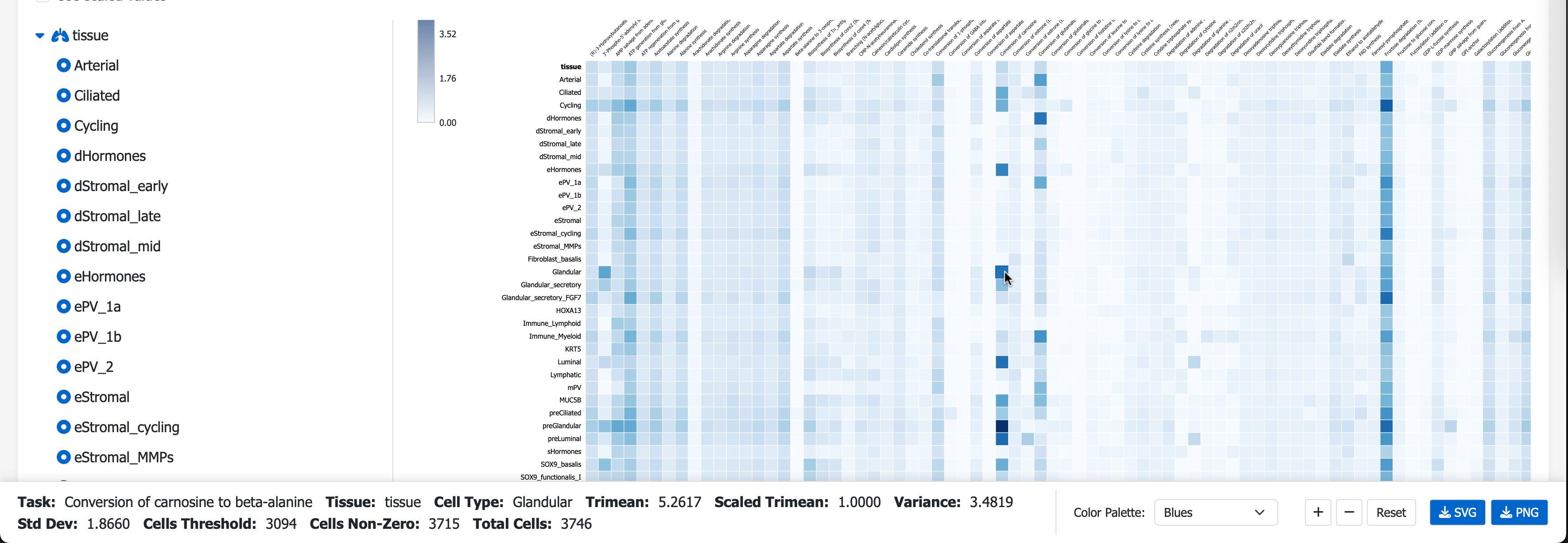
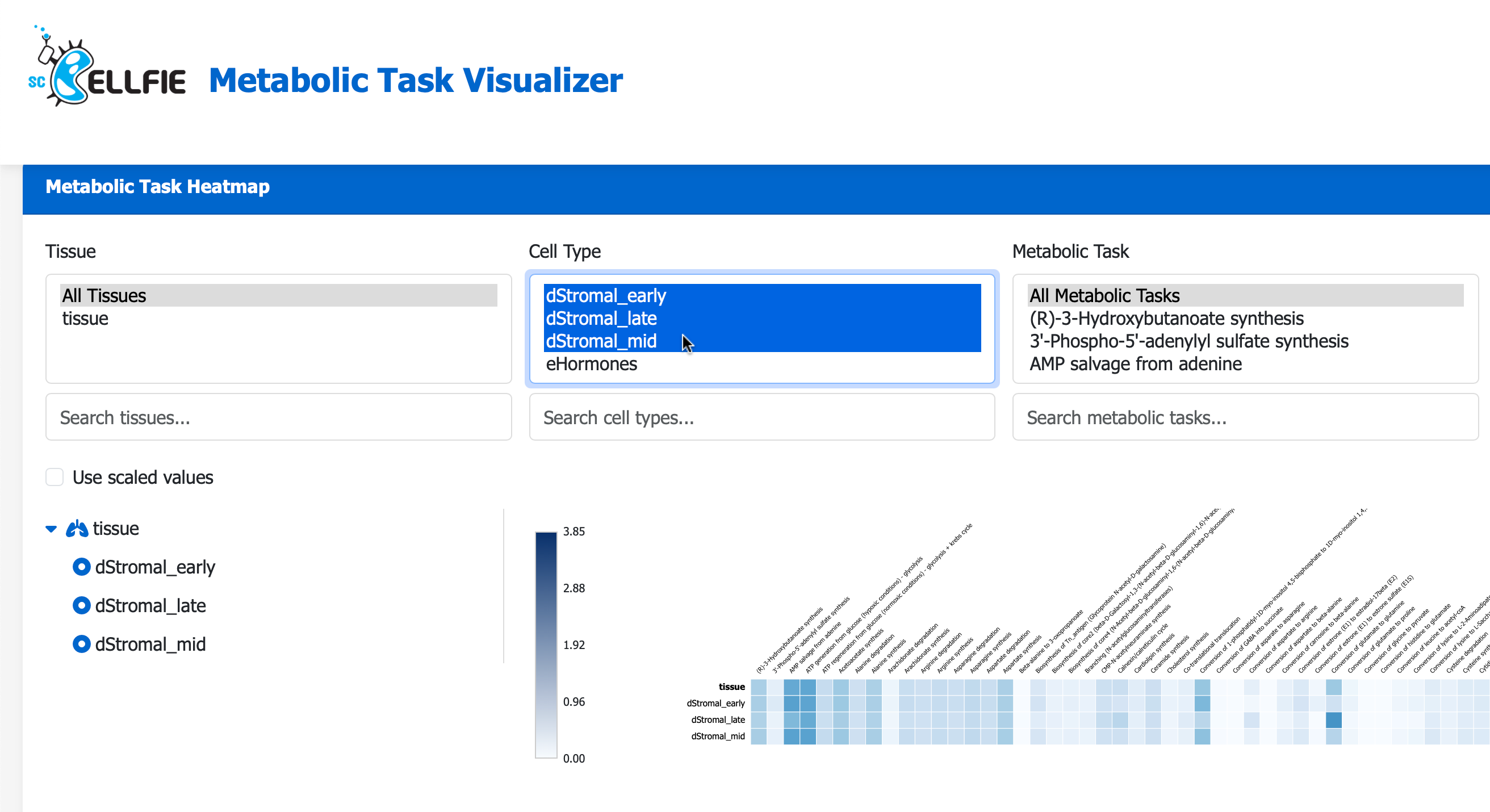
Next, visit the scCellFie Metabolic Task Visualizer portal, you can Drag N’ Drop your saved Melted.csv to visualise the result in a heatmap.

Additional local visualizations

These outputs can be further used to visualize metabolic task activities with a radial plot. In this case, all cell types within the tissue are included. The maximum activity per task, across all cell types, is shown.

fig, ax = sccellfie.plotting.create_radial_plot(melted, results['task_info'], figsize=(6,6), sort_by_value=False, ylim=1.0)

Or we can also plot the activities of each cell type:

# Create figure with subplots
fig = plt.figure(figsize=(16, 16))
ax1 = fig.add_subplot(221, projection='polar')
ax2 = fig.add_subplot(222, projection='polar')
ax3 = fig.add_subplot(223, projection='polar')
ax4 = fig.add_subplot(224, projection='polar')

for i, (cell, ax) in enumerate(zip(['eStromal', 'dStromal_early', 'dStromal_mid', 'dStromal_late'], [ax1, ax2, ax3, ax4])):
    sccellfie.plotting.create_radial_plot(melted,
                                          results['task_info'],
                                          cell_type=cell,
                                          ax=ax,
                                          show_legend=i == 1,
                                          ylim=1.0
                                          )