Communication (single-cell)

In this tutorial, we will walk you through how to infer metabolite-mediated cell-cell communication using single-cell data.

Here, we will use the results we previously generated for the Human Endometrial Cell Atlas (HECA) dataset (Mareckova & Garcia-Alonso et al 2023) by running our Quick Start Tutorial.

This tutorial includes following steps:

• Loading libraries

• Loading endometrium results

• Defining cell types

• Data preparation

• Inferring intercellular communication

• Visualizing interactions

Loading libraries

import sccellfie
import scanpy as sc

import pandas as pd
import numpy as np

import matplotlib.pyplot as plt
import seaborn as sns
import glasbey

import textwrap

## To avoid warnings
import warnings
warnings.filterwarnings("ignore")

In addition, we set up a folder to save our figures. This folder is stored in the settings of Scanpy:

sc.settings.figdir = './results/communication-figures/'

Loading endometrium results

We start opening the results previously generated by running the scCellFie pipeline on the HECA dataset. If you haven’t run the pipeline yet, please follow this tutorial.

In this case, we will load the objects that were present in results['adata'] in that tutorial. This object contains:

• results['adata']: contains gene expression in .X.

• results['adata'].layers['gene_scores']: contains gene scores as in the original CellFie paper.

• results['adata'].uns['Rxn-Max-Genes']: contains determinant genes for each reaction per cell.

• results['adata'].reactions: contains reaction scores in .X so every scanpy function can be used on this object to visualize or compare values.

• results['adata'].metabolic_tasks: contains metabolic task scores in .X so every scanpy function can be used on this object to visualize or compare values.

Here, we will name this object directly as adata. Each of the previous elements should be under adata., as for example adata.metabolic_tasks.

adata = sccellfie.io.load_adata(folder='./results/',
                                filename='Human_HECA_scCellFie'
                               )

./results//Human_HECA_scCellFie.h5ad was correctly loaded
./results//Human_HECA_scCellFie_reactions.h5ad was correctly loaded
./results//Human_HECA_scCellFie_metabolic_tasks.h5ad was correctly loaded

In this case, we are interested in the metabolic task scores, which can be found in the adata.metabolic_tasks AnnData object.

adata.metabolic_tasks

AnnData object with n_obs × n_vars = 90001 × 215
    obs: 'n_genes', 'sample', 'percent_mito', 'n_counts', 'Endometriosis_stage', 'Endometriosis', 'Hormonal treatment', 'Binary Stage', 'Stage', 'phase', 'dataset', 'Age', 'lineage', 'celltype', 'label_long'
    uns: 'Binary Stage_colors', 'Biopsy_type_colors', 'Endometrial_pathology_colors', 'Endometriosis_stage_colors', 'GarciaAlonso_celltype_colors', 'Group_colors', 'Hormonal treatment_colors', 'Library_genotype_colors', 'Mareckova_celltype_colors', 'Mareckova_epi_celltype_colors', 'Mareckova_lineage_colors', 'Processing_colors', 'Symbol_colors', 'Tan_cellsubtypes_colors', 'Tan_celltype_colors', 'Treatment_colors', 'celltype_colors', 'dataset_colors', 'genotype_colors', 'hvg', 'label_long_colors', 'leiden', 'leiden_R_colors', 'leiden_colors', 'lineage_colors', 'neighbors', 'normalization', 'phase_colors', 'umap'
    obsm: 'X_scVI', 'X_umap'
    obsp: 'connectivities', 'distances'

Defining cell types

For metabolic marker identification, we need to specify which column in the AnnData object contains the cell type information:

# Our column indicating the cell types in the adata.obs dataframe
cell_group = 'celltype'

Which can be visualized as

sc.pl.umap(adata, color=cell_group, frameon=False)

Data preparation

scCellFie generates separate AnnData objects containing either reaction scores (adata.reactions) or task scores (adata.metabolic_tasks). Therefore, to infer cell-cell communication, we need to put metabolic task scores together with gene expression in the same AnnData object.

We load our subset of the HECA data, where gene expression of all genes is contained:

bdata = sc.read(filename='./data/HECA-Subset.h5ad',
                backup_url='https://zenodo.org/records/15072628/files/HECA-Subset.h5ad')

Then, we transform gene expression into log1p(CP10k) values.

sc.pp.normalize_total(bdata, target_sum=10000)
sc.pp.log1p(bdata)

We assign a ‘type’ column for the features in each AnnData, so we can easily recognize which are genes and tasks.

adata.metabolic_tasks.var['type'] = 'metabolic score'
bdata.var['type'] = 'gene expression'

Here, we transfer metabolic scores into the AnnData object containing gene expression. For this, we use a built-in function in scCellFie to transfer features from one source adata into another target adata. In this case we transfer all metabolic tasks (by using var_names=adata.metabolic_tasks.var_names).

adata_updated = sccellfie.preprocessing.adata_utils.transfer_variables(
    adata_target=bdata,
    adata_source=adata.metabolic_tasks,
    var_names=adata.metabolic_tasks.var_names
)

adata_updated

AnnData object with n_obs × n_vars = 90001 × 17951
    obs: 'n_genes', 'sample', 'percent_mito', 'n_counts', 'Endometriosis_stage', 'Endometriosis', 'Hormonal treatment', 'Binary Stage', 'Stage', 'phase', 'dataset', 'Age', 'lineage', 'celltype', 'label_long'
    var: 'type'
    uns: 'Binary Stage_colors', 'Biopsy_type_colors', 'Endometrial_pathology_colors', 'Endometriosis_stage_colors', 'GarciaAlonso_celltype_colors', 'Group_colors', 'Hormonal treatment_colors', 'Library_genotype_colors', 'Mareckova_celltype_colors', 'Mareckova_epi_celltype_colors', 'Mareckova_lineage_colors', 'Processing_colors', 'Symbol_colors', 'Tan_cellsubtypes_colors', 'Tan_celltype_colors', 'Treatment_colors', 'celltype_colors', 'dataset_colors', 'genotype_colors', 'hvg', 'label_long_colors', 'leiden', 'leiden_R_colors', 'leiden_colors', 'lineage_colors', 'neighbors', 'phase_colors', 'umap', 'log1p'
    obsm: 'X_scVI', 'X_umap'
    obsp: 'connectivities', 'distances'

Inferring intercellular communication

Using our new AnnData object (adata_updated), we can infer cell-cell communication by computing communication scores (see this review paper for more details) for a list of ligand-receptor (LR) pairs.

Defining list of LR pairs

In this case, our ligand is represented by the metabolic task(s) that produce this metabolite, while the receptor is the gene encoding for the known protein that interacts with the ligand.

Here we define a few LR pairs:

lr_pairs = [('Synthesis of estradiol-17beta (E2) from androstenedione', 'ESR1'),
            ('Synthesis of L-kynurenine from tryptophan', 'AHR'),
            ('Synthesis of thromboxane from arachidonate', 'TBXA2R'),
           ]

If you are interested in other interactions, you can always define your own LR pairs based on the metabolic tasks present in scCellFie’s metabolic database.

Note!

scCellFie now supports the inclusion of “complexes” either for the ligand or for the receptor. For example we can pass a receptor made of multiple subunits, or multiple metabolic tasks in case we can to consider all steps for synthesizing a given metabolite, but we need to add them to our adata_updated:

# Add complexes for multi-subunit receptors or multi-task metabolic elements
complexes = {
    'taskA&taskB': ['taskA', 'taskB'],       # multiple tasks producing same metabolite
    'GENE1&GENE2': ['GENE1', 'GENE2'],       # receptor complex subunits
}

# This function makes the magic of including the complexes defined before
sccellfie.preprocessing.add_complexes_to_adata(adata_updated, complexes, agg_method='min')

# Use complex names alongside regular LR pairs
# Ligands can be metabolic tasks or genes (e.g., secreted proteins)
lr_pairs = [
    ('taskA&taskB', 'GENE1&GENE2'),   # complex task ligand -> complex receptor
    ('taskC', 'GENE3'),                # single task ligand -> single receptor
    ('GENE4', 'GENE5'),               # single gene ligand -> single receptor
    ('GENE4', 'GENE1&GENE2'),         # single gene ligand -> complex receptor
]

Computing communication scores

In this case we use the geometric mean between the cell-type level aggregated values (using the Tuckey’s trimean). For the ligand we use the metabolic score of the corresponding metabolic task, while for the receptor we use the log-transformed gene expression (log1p(CP10k)).

ccc_df = sccellfie.communication.compute_communication_scores(adata_updated,
    var_pairs=lr_pairs,
    groupby=cell_group,
    communication_score='gmean',
    agg_func='trimean',
    ligand_threshold=np.log(2), # Greater than this metabolic activity for considering it active
    receptor_threshold=0., # Greater than this expression for considering it active
)

Our communication scores are in the 'score' columm of the ccc_df. Additionlly, this dataframe contains the fraction of cells expressing the ligand, and the receptor. These fractions were calculated as the cells with the metabolic score greater than the ligand_threshold with respect the total of cells in a cell type. Similarly, the fraction was calculated for the receptor, based on the receptor_threshold value.

ccc_df.head()

	sender_celltype	receiver_celltype	ligand	receptor	score	ligand_fraction	receptor_fraction
0	Arterial	Arterial	Synthesis of estradiol-17beta (E2) from andros...	ESR1	0.000000	0.082136	0.057495
1	Arterial	Arterial	Synthesis of L-kynurenine from tryptophan	AHR	0.201260	0.088296	0.605749
2	Arterial	Arterial	Synthesis of thromboxane from arachidonate	TBXA2R	0.000000	0.110883	0.188912
3	Arterial	Ciliated	Synthesis of estradiol-17beta (E2) from andros...	ESR1	0.447837	0.082136	0.712575
4	Arterial	Ciliated	Synthesis of L-kynurenine from tryptophan	AHR	0.090771	0.088296	0.459747

Other cell-cell communication tools

As you can see, here we do not compute P-values since we do not perform any statistical analysis (e.g. permutation analysis).

Other tools already implement this kind of analysis (e.g. CellPhoneDB and LIANA), so we can export our unified AnnData object to run the analysis with another tool.

We can save this new object:

adata_updated.write_h5ad('./results/CCC-Endometrium.h5ad')

Similarly, we can output our database of LR pairs:

lr_df = pd.DataFrame.from_records(lr_pairs, columns=['ligand', 'receptor'])
lr_df

	ligand	receptor
0	Synthesis of estradiol-17beta (E2) from andros...	ESR1
1	Synthesis of L-kynurenine from tryptophan	AHR
2	Synthesis of thromboxane from arachidonate	TBXA2R

We can additionally define shorter names for our LR pairs:

lr_names = ['E2 - ESR1',
            'Kynurenine - AHR',
            'Thromboxane - TBXA2R']

lr_df['lr_name'] = lr_names
lr_df

	ligand	receptor	lr_name
0	Synthesis of estradiol-17beta (E2) from andros...	ESR1	E2 - ESR1
1	Synthesis of L-kynurenine from tryptophan	AHR	Kynurenine - AHR
2	Synthesis of thromboxane from arachidonate	TBXA2R	Thromboxane - TBXA2R

lr_df.to_csv('./results/LR-Pairs.csv', index=False)

Note!

Please make sure to format this data in the proper way for the tool you plan using.

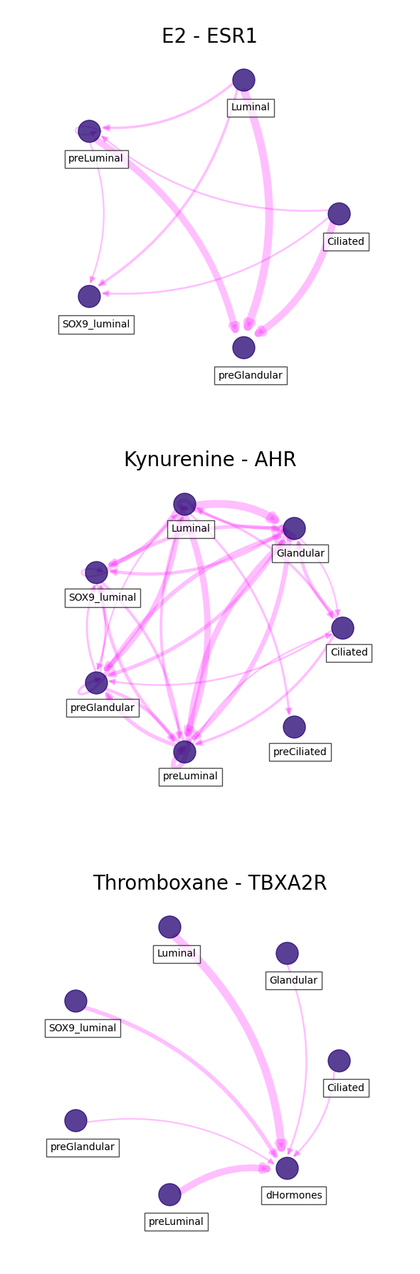
Visualizing interactions

In this case we can visualize each of the ligand-receptor interactions we passed.

For clear visualizations, we can filter important interactions based on the 'score', 'ligand_fraction' and 'receptor_fraction'. Additionally, we can define a specific list of cell types to include:

celltypes = ['SOX9_luminal', 'preLuminal', 'Luminal',
             'preCiliated', 'Ciliated', 'dHormones',
             'preGlandular', 'Glandular', 'Glandular secretory',
             'dStromal_early', 'dStromal_mid', 'dStromal_late']

fig, axs = plt.subplots(len(lr_pairs),
                        1,
                        figsize = (6, 6 * len(lr_pairs)))

axes = axs.flatten()

for i, lr in enumerate(lr_pairs):
    df = ccc_df.loc[(ccc_df.ligand == lr[0]) & (ccc_df.receptor == lr[1])]

    # THRESHOLD FOR IMPORTANT COMMUNICATION SCORE IS MEAN + 1 STD
    score_thresh = df.score.mean() + df.score.std()

    # CELL TYPES MUST EXPRESS LIGAND AND RECEPTOR IN MORE THAN 10% OF SINGLE CELLS
    frac_thresh = (df.ligand_fraction > 0.1) & (df.receptor_fraction > 0.1)

    # FILTER INTERACTONS
    filtered_df = df.loc[(df.score >= score_thresh) & (frac_thresh)]

    # INCLUDE SPECIFIC CELL TYPES
    filtered_df = filtered_df.loc[(filtered_df.sender_celltype.isin(celltypes)) \
                                  & (filtered_df.receiver_celltype.isin(celltypes))]

    # PLOT INTERACTIONS
    ax = axes[i]
    sccellfie.plotting.plot_communication_network(filtered_df,
                                                  'sender_celltype',
                                                  'receiver_celltype',
                                                  'score',
                                                  panel_size=(6,6),
                                                  network_layout='circular',
                                                  edge_color='magenta',
                                                  edge_width=8,
                                                  edge_arrow_size=12,
                                                  edge_alpha=0.25,
                                                  node_color='#210070',
                                                  node_size=500,
                                                  node_alpha=0.75,
                                                  node_label_size=10,
                                                  node_label_alpha=0.7,
                                                  node_label_offset=(0.05, -0.2),
                                                  title=lr_names[i],
                                                  title_fontsize=20,
                                                  tight_layout=True,
                                                  ax=ax
                                                 )