Differential Analysis
![]()
In this tutorial, we will walk you through how to perform a differential analysis for identifying changes in the metabolic task scores between two conditions.
Here, we will use the results we previously generated for the Human Endometrial Cell Atlas (HECA) dataset (Mareckova & Garcia-Alonso et al 2023) by running our Quick Start Tutorial.
This tutorial includes following steps:
Loading libraries
[1]:
import sccellfie
import scanpy as sc

import pandas as pd
import numpy as np

import matplotlib.pyplot as plt
import seaborn as sns
import glasbey

import textwrap

import os
import re

## To avoid warnings
import warnings
warnings.filterwarnings("ignore")
/home/jovyan/my-conda-envs/single_cell/lib/python3.10/site-packages/dask/dataframe/__init__.py:31: FutureWarning: The legacy Dask DataFrame implementation is deprecated and will be removed in a future version. Set the configuration option `dataframe.query-planning` to `True` or None to enable the new Dask Dataframe implementation and silence this warning.
  warnings.warn(
In addition, we set up a folder to save our figures. This folder is stored in the settings of Scanpy:
[2]:
sc.settings.figdir = './results/da-figures/'
[3]:
os.makedirs(sc.settings.figdir, exist_ok=True)
Loading endometrium results
We start opening the results previously generated by running the scCellFie pipeline on the HECA dataset. If you haven’t run the pipeline yet, please follow this tutorial.
In this case, we will load the objects that were present in results['adata'] in that tutorial. This object contains:
results['adata']: contains gene expression in.X.results['adata'].layers['gene_scores']: contains gene scores as in the original CellFie paper.results['adata'].uns['Rxn-Max-Genes']: contains determinant genes for each reaction per cell.results['adata'].reactions: contains reaction scores in.Xso every scanpy function can be used on this object to visualize or compare values.results['adata'].metabolic_tasks: contains metabolic task scores in.Xso every scanpy function can be used on this object to visualize or compare values.
Here, we will name this object directly as adata. Each of the previous elements should be under adata., as for example adata.metabolic_tasks.
[4]:
adata = sccellfie.io.load_adata(folder='./results/',
                                filename='Human_HECA_scCellFie'
                               )
./results//Human_HECA_scCellFie.h5ad was correctly loaded
./results//Human_HECA_scCellFie_reactions.h5ad was correctly loaded
./results//Human_HECA_scCellFie_metabolic_tasks.h5ad was correctly loaded
In this case, we are interested in the metabolic task scores, which can be found in the adata.metabolic_tasks AnnData object.
[5]:
adata.metabolic_tasks
[5]:
AnnData object with n_obs × n_vars = 90001 × 215
    obs: 'n_genes', 'sample', 'percent_mito', 'n_counts', 'Endometriosis_stage', 'Endometriosis', 'Hormonal treatment', 'Binary Stage', 'Stage', 'phase', 'dataset', 'Age', 'lineage', 'celltype', 'label_long'
    uns: 'Binary Stage_colors', 'Biopsy_type_colors', 'Endometrial_pathology_colors', 'Endometriosis_stage_colors', 'GarciaAlonso_celltype_colors', 'Group_colors', 'Hormonal treatment_colors', 'Library_genotype_colors', 'Mareckova_celltype_colors', 'Mareckova_epi_celltype_colors', 'Mareckova_lineage_colors', 'Processing_colors', 'Symbol_colors', 'Tan_cellsubtypes_colors', 'Tan_celltype_colors', 'Treatment_colors', 'celltype_colors', 'dataset_colors', 'genotype_colors', 'hvg', 'label_long_colors', 'leiden', 'leiden_R_colors', 'leiden_colors', 'lineage_colors', 'neighbors', 'normalization', 'phase_colors', 'umap'
    obsm: 'X_scVI', 'X_umap'
    obsp: 'connectivities', 'distances'
Defining cell types
For metabolic marker identification, we need to specify which column in the AnnData object contains the cell type information:
[6]:
# Our column indicating the cell types in the adata.obs dataframe
# Here, label_long contains the full name of cell types.
# Shorter names can be found under the celltype column
cell_group = 'label_long'
Which can be visualized as
[7]:
sc.pl.umap(adata, color=cell_group, frameon=False)

Differential analysis
We can perform a differential analysis to identify changes between two conditions (per cell type). In this case, we focus on donors with and without endometriosis
Select conditions to compare
[8]:
adata.obs.Endometriosis.unique()
[8]:
['Control', 'Endometriosis']
Categories (2, object): ['Control', 'Endometriosis']
[9]:
contrasts = [('Control', 'Endometriosis')]
condition_key = 'Endometriosis'
Filter testable cell types (optional)
Additionally, we can filter cell types to test. This may be useful to increase statistical power as in some cases, for a given cell type, one condition could have substantially more single cells than the other, affecting the results.
In this case we can filter by:
Number of minimum cells per cell type
Ratio of single cells between conditions
[10]:
# Here, we pick celltype column for the counts, but this doesn't matter as all columns will have the same counts.
control_cells = adata.metabolic_tasks.obs.groupby(['Endometriosis', cell_group])['celltype'].count().loc['Control']
endo_cells = adata.metabolic_tasks.obs.groupby(['Endometriosis', cell_group])['celltype'].count().loc['Endometriosis']
[11]:
# Filters
min_n = 50 # Here we do not use a big number as we are only using a subset of the original dataset.
max_log2ratio = 6 # This is 2 power 6 (or 64)

testable_cells = control_cells.index[(control_cells >= min_n) & (endo_cells >= min_n) & (np.log2(control_cells / endo_cells).abs() <= max_log2ratio)].tolist()
[12]:
testable_cells
[12]:
['3 | SOX9 functionalis II',
 '4 | SOX9 luminal',
 '5 | Cycling',
 '6 | preGlandular',
 '7 | Glandular',
 '8 | Glandular secretory',
 '10 | preLuminal',
 '11 | Luminal',
 '12 | preCiliated',
 '13 | Ciliated',
 '14 | MUC5B',
 '16 | eHormones',
 '20 | ePV 1b',
 '21 | ePV 2',
 '22 | eStromal MMPs',
 '23 | eStromal',
 '24 | eStromal cycling',
 '25 | dStromal early',
 '26 | dStromal mid',
 '27 | dStromal late',
 '29 | HOXA13',
 '30 | sHormones',
 '32 | Venous',
 '33 | Arterial',
 '35 | Immune Lymphoid',
 '36 | Immune Myeloid']
In case you do not want to filter testable cells, just leave input_adata = adata.metabolic_tasks.
We can also test individual reactions instead of metabolic tasks; in that case, use adata.reactions.
[13]:
input_adata = adata.metabolic_tasks[adata.metabolic_tasks.obs['label_long'].isin(testable_cells)]
Perform differential analysis
scCellFie implements a Wilcoxon rank sum test (a.k.a. Mann-Whitney U test) by using the Scanpy’s implementation. However, other differential analyses could be performed by using external tools. For example, Pertpy offers multiple options. Advanced users can implement their own GLMs by using statsmodels.
[14]:
de_results = sccellfie.stats.scanpy_differential_analysis(input_adata,
                                                          cell_type=None,
                                                          cell_type_key=cell_group,
                                                          condition_key=condition_key,
                                                          min_cells=0, # We do not use this as we already filtered cells before
                                                          condition_pairs=contrasts)
Processing DE analysis: 100%|██████████| 26/26 [01:11<00:00, 2.76s/it]
Results interpretation and visualization
Once we have our results, the first thing we can do it’s to export them:
[15]:
de_results.reset_index().to_csv(f'{sc.settings.figdir}/DE-Endometriosis.csv')
When inspecting our results, we find multiple columns containing useful information:
cell_type: The annotated cell type in which the differential analysis was performed, in this case corresponds to the column'long_label'in theinput_adata.obsdataframe.feature: The metabolic task evaluated for differential activity. This could be reactions or genes depending on the AnnData object used as input.group1andgroup2: The two biological conditions or groups being compared.log2FC: The log2 fold-change in metabolic activity between group2 and group1, where positive values indicate higher activity in group2. Here the mean activity in each group-cell type is used.test_statistic: The value of the test statistic used for assessing significance (e.g., from a Wilcoxon or t-test).p_value: The unadjusted p-value indicating the likelihood of observing this result by chance.cohens_d: The effect size (Cohen’s D), which quantifies the difference between two means (from each group) divided by a standard deviation for the data. Positive values indicate higher mean in group2, while negative values indicate higher mean in group1.n_group1andn_group2: The number of cells in group1 and group2, respectively, used in the comparison.median_group1andmedian_group2: The median inferred metabolic activity for the feature in group1 and group2, respectively.median_diff: The difference in median values between group2 and group1.adj_p_value: The p-value adjusted for multiple testing, typically using the Benjamini-Hochberg FDR correction.
[16]:
de_results.head()
[16]:
| cell_type | feature | group1 | group2 | log2FC | test_statistic | p_value | cohens_d | n_group1 | n_group2 | median_group1 | median_group2 | median_diff | adj_p_value | |
|---|---|---|---|---|---|---|---|---|---|---|---|---|---|---|
| 0 | 33 | Arterial | Synthesis of inositol | Control | Endometriosis | 0.255916 | 6.212417 | 5.217592e-10 | 0.601413 | 332 | 155 | 2.931521848895364 | 3.497998206239549 | 0.566476 | 1.677190e-09 |
| 1 | 33 | Arterial | Glucuronate synthesis (via inositol) | Control | Endometriosis | 0.255861 | 6.206195 | 5.428279e-10 | 0.601341 | 332 | 155 | 2.1986413866715226 | 2.6234986546796617 | 0.424857 | 1.743913e-09 |
| 2 | 33 | Arterial | Calnexin/calreticulin cycle | Control | Endometriosis | 0.406157 | 4.629761 | 3.660886e-06 | 0.474405 | 332 | 155 | 0.6617462596432262 | 0.9516740021385109 | 0.289928 | 8.963798e-06 |
| 3 | 33 | Arterial | Galactosylation (addition of galactose) | Control | Endometriosis | 0.372435 | 4.542661 | 5.554853e-06 | 0.184975 | 332 | 155 | 0.05415647236936193 | 0.09829356067435617 | 0.044137 | 1.333833e-05 |
| 4 | 33 | Arterial | Reactive oxygen species detoxification (H2O2 t... | Control | Endometriosis | 0.878627 | 3.487096 | 4.882954e-04 | 0.499638 | 332 | 155 | 0.08105852111581638 | 0.17828518585456787 | 0.097227 | 9.604403e-04 |
Visualizations
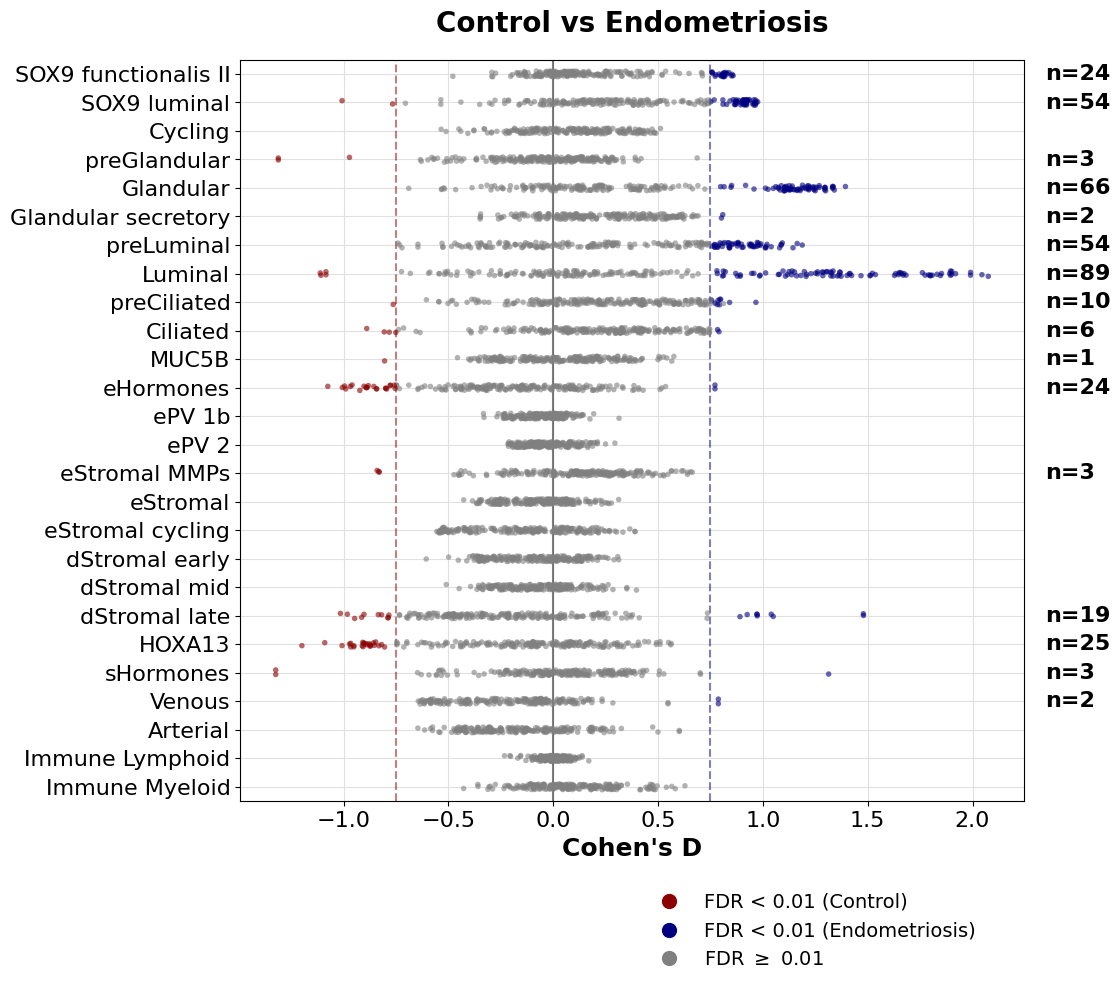
We can use a beeswarm plot, where each row (y-axis) represents the cell types, and the x-axis shows the effect size. Dots are each of the tested features (metabolic tasks), and colored whether they pass both filters, adj. P value and effect size (Cohen’s D here).
To understand this plot, each row can be seen as a “flattened volcano plot”.
We first set some filter to call a result significant:
[17]:
cohen_threshold = 0.75 # Min value of absolute Cohen's D.
pval_threshold = 0.01 # Min adj. P value
logfc_threshold = np.log2(1.1) # Min log2FC. Leave it as np.log2(1.) if you do not want to use this filter
We can pass a function to sort cells in the y-axis. This function is to sort them by they cluster number:
[18]:
sort_lambda = lambda x: pd.Series([int(s.split(' | ')[0]) for s in x])
[19]:
fig, ax, sig = sccellfie.plotting.create_beeswarm_plot(de_results,
                                                       x='cohens_d',
                                                       cohen_threshold=cohen_threshold,
                                                       pval_threshold=pval_threshold,
                                                       logfc_threshold=logfc_threshold,
                                                       show_n_significant=True, # To indicate the number of significant features at the right of the plot
                                                       strip_jitter=True,
                                                       sort_lambda=sort_lambda,
                                                       lgd_bbox_to_anchor=(0.5, -0.1), # Location of the legend
                                                       ticks_fontsize=16,
                                                       labels_fontsize=18,
                                                       figsize=(12, 10), )

# Remove cluster number (optional)
ylabels = ax.get_yticklabels()
ax.set_yticklabels([t.get_text().split(' | ')[1] for t in ylabels])
ax.set_ylabel('')

plt.savefig(f'{sc.settings.figdir}/Endometriosis-DE.pdf', dpi=300, bbox_inches='tight')
The number of unique metabolic tasks changing across all cell types:
[20]:
sig_tasks = sig.reset_index().feature.unique().tolist()
len(sig_tasks)
[20]:
115
Alternatively, we can use a volcano plot for one cell type at a time.
[21]:
luminal_tasks = sccellfie.plotting.create_volcano_plot(de_results,
                                                       effect_threshold=0.75,
                                                       padj_threshold=0.05,
                                                       cell_type='11 | Luminal',
                                                       group1=None,
                                                       group2=None,
                                                       effect_col='cohens_d',
                                                       effect_title="Cohen's d",
                                                       wrapped_title_length=50,
                                                       save='Overall-VolcanoPlot',
                                                       dpi=300,
                                                       tight_layout=True
                                                      )

[22]:
len(luminal_tasks)
[22]:
89
Plot number of major task groups up/down regulated
We use our outputs from scCellFie to calculate the number of significant tasks given their major categories located in sccellfie_db['task_info'], after downloading the scCellFie’s database:
[23]:
sccellfie_db = sccellfie.datasets.load_sccellfie_database(organism='human')
We define our function to make a plot showing these numbers
[24]:
def plot_single(condition, ax, pathway, sig_data):
    pathway_counts = {'System': pd.DataFrame(), 'Subsystem': pd.DataFrame()}

    for c, df in sig_data.reset_index().groupby('cell_type'):
        for k, v in pathway_counts.items():
            df2 = df.set_index('feature').join(sccellfie_db['task_info'].set_index('Task'), how='inner')
            df2 = df2.loc[df2.log2FC > 0] if condition == 'up' else df2.loc[df2.log2FC < 0]
            df2 = df2.value_counts(k).to_frame().reset_index()
            df2['cell_type'] = c
            df2 = df2[['cell_type', k, 'count']]
            df2[k] = df2[k].apply(lambda x: x.upper())
            pathway_counts[k] = pd.concat([pathway_counts[k], df2])

    df = pathway_counts[pathway].sort_values('count')
    totals = df.groupby('cell_type')['count'].sum()

    df_normalized = df.copy()
    df_normalized['fraction'] = df.groupby('cell_type')['count'].transform(lambda x: x / x.sum())
    pivoted_data = df_normalized.pivot(index='cell_type', columns=pathway, values='fraction')
    pivoted_data = pivoted_data.sort_index().fillna(0.)

    n_systems = len(pivoted_data.columns)
    colors = glasbey.extend_palette('Set2', palette_size=max([n_systems, 10]))

    pivoted_data.plot(kind='barh', stacked=True, ax=ax, color=colors, legend=False)
    ax.set_xlim((0, 1))
    ax.invert_yaxis()

    ylabels = ax.get_yticklabels()
    ax.tick_params(axis='both', which='major', labelsize=12)

    for idx, cell_type in enumerate(pivoted_data.index):
        ax.text(1.02, idx, f'n={totals[cell_type]:,}', va='center', fontsize=12)

    ax.set_xlabel('Fraction', fontsize=14)
    ax.set_ylabel('')

    return pivoted_data.columns, colors
Then we plot these numbers
[25]:
from matplotlib.colors import to_rgb

pathway = 'System'
condition1_color='#8B0000'
condition2_color='#000080'
fig, (ax1, ax2) = plt.subplots(2, 1, figsize=(6, 12), height_ratios=[1, 1])

legend_elements, colors = plot_single('up', ax1, pathway, sig)
plot_single('down', ax2, pathway, sig)

ax1.set_title('Endometriosis', fontsize=16, pad=10, color=to_rgb(condition2_color))
ax2.set_title('Control', fontsize=16, pad=10, color=to_rgb(condition1_color))

plt.figlegend(labels=legend_elements,
              bbox_to_anchor=(0.5, -0.005),
              ncols=2 if pathway == 'System' else 2,
              frameon=False,
              loc='upper center')

plt.subplots_adjust(hspace=0.5)
# For saving this figure, uncomment the code below
# plt.savefig(f'{sc.settings.figdir}./scCellFie-DA-{pathway}-Combined.pdf',
#             dpi=300,
#             bbox_inches='tight')

Visualize changes in distributions across single cells
For the significant tasks, we can also compare their distribution of metabolic scores for each condition.
[26]:
cell_show = ['7 | Glandular', '11 | Luminal',]

for c in cell_show:
    sig_features = [idx for idx in sig.loc[c].sort_values('log2FC').index]
    N = len(sig_features)
    if N > 0:
        width = min([18, 1.5 + 0.5*N])
        fig, ax = sccellfie.plotting.create_comparative_violin(adata=adata.metabolic_tasks,
                                                               significant_features=sig_features,
                                                               group1='Control',
                                                               group2='Endometriosis',
                                                               condition_key=condition_key,
                                                               cell_type_key=cell_group,
                                                               celltype=c,
                                                               xlabel='',
                                                               ylabel='Metabolic Score',
                                                               palette=['coral','cornflowerblue'],
                                                               wrapped_title_length=100,
                                                               figsize=(width, 4),
                                                               fontsize=14,
                                                               title=c,
                                                               tight_layout=False,
                                                               #save=f'DE-Dist-{cname}'
                                                              )


Additional differential analysis
Another analysis in scCellFie is a differential analysis comparing each metabolic task between conditions, using all single cells. In contrast, the analysis shown in the previous sections performs it in a cell-type-wise manner. Here, we also use a Wilcoxon rank sum test.
[27]:
da_all = sccellfie.stats.pairwise_differential_analysis(adata.metabolic_tasks,
                                                        groupby='Endometriosis', # Column including the conditions
                                                        var_names=None,
                                                        order=None,
                                                        alternative='two-sided',
                                                        alpha=0.05)
Processing features: 100%|██████████| 215/215 [00:02<00:00, 73.89it/s]
The columns here are consistent with the previous analysis, but the cell_type column is not included:
feature: The metabolic task evaluated for differential activity. This could be reactions or genes depending on the AnnData object used as input.group1andgroup2: The two biological conditions or groups being compared.log2FC: The log2 fold-change in metabolic activity between group2 and group1, where positive values indicate higher activity in group2. Here the mean activity in each group-cell type is used.test_statistic: The value of the test statistic used for assessing significance (e.g., from a Wilcoxon or t-test).p_value: The unadjusted p-value indicating the likelihood of observing this result by chance.cohens_d: The effect size (Cohen’s D), which quantifies the difference between two means (from each group) divided by a standard deviation for the data. Positive values indicate higher mean in group2, while negative values indicate higher mean in group1.n_group1andn_group2: The number of cells in group1 and group2, respectively, used in the comparison.median_group1andmedian_group2: The median inferred metabolic activity for the feature in group1 and group2, respectively.median_diff: The difference in median values between group2 and group1.adj_p_value: The p-value adjusted for multiple testing, typically using the Benjamini-Hochberg FDR correction.
[28]:
da_all.head()
[28]:
| feature | group1 | group2 | log2FC | test_statistic | p_value | cohens_d | n_group1 | n_group2 | median_group1 | median_group2 | median_diff | adj_p_value | |
|---|---|---|---|---|---|---|---|---|---|---|---|---|---|
| 0 | (R)-3-Hydroxybutanoate synthesis | Control | Endometriosis | 0.007330 | -3.490743 | 4.816790e-04 | 0.014760 | 48350 | 41651 | 1.504349 | 1.475321 | -0.029028 | 6.638525e-04 |
| 1 | 3'-Phospho-5'-adenylyl sulfate synthesis | Control | Endometriosis | -0.215446 | -22.884917 | 6.566557e-116 | -0.128798 | 48350 | 41651 | 0.630853 | 0.515172 | -0.115681 | 6.722904e-115 |
| 2 | AMP salvage from adenine | Control | Endometriosis | 0.058398 | 10.906711 | 1.070605e-27 | 0.071603 | 48350 | 41651 | 2.078593 | 2.176834 | 0.098241 | 2.951026e-27 |
| 3 | ATP generation from glucose (hypoxic condition... | Control | Endometriosis | 0.013908 | -2.080721 | 3.745946e-02 | 0.027402 | 48350 | 41651 | 2.411501 | 2.369780 | -0.041721 | 4.306836e-02 |
| 4 | ATP regeneration from glucose (normoxic condit... | Control | Endometriosis | -0.034165 | -17.806112 | 6.336087e-71 | -0.073807 | 48350 | 41651 | 1.082905 | 1.024853 | -0.058052 | 3.584891e-70 |
Volcano plot
[29]:
overall_tasks = sccellfie.plotting.create_volcano_plot(da_all,
                                                       effect_threshold=0.25,
                                                       padj_threshold=0.05,
                                                       cell_type=None,
                                                       group1=None,
                                                       group2=None,
                                                       effect_col='cohens_d',
                                                       effect_title="Cohen's d",
                                                       wrapped_title_length=50,
                                                       save='Overall-VolcanoPlot',
                                                       dpi=300,
                                                       tight_layout=True
                                                      )

[30]:
len(overall_tasks)
[30]:
7
[31]:
overall_tasks
[31]:
['Synthesis of anthranilate from tryptophan',
 'Degradation of guanine to urate',
 'Synthesis of L-kynurenine from tryptophan',
 'Synthesis of kynate from tryptophan',
 'Synthesis of N-formylanthranilate from tryptophan',
 'Synthesis of quinolinate from tryptophan',
 'Mevalonate synthesis']