General Overview
![]()
This notebook provides a general overview of scCellFie analyses, including the inference of metabolic tasks, metabolic marker identification, differential analysis, and cell-cell communication.
To illustrate a different application, the dataset we are using here includes BALF samples from donors with varying severities of COVID-19 (Liao et al 2020).
This tutorial includes following steps:
Loading libraries
[ ]:
import sccellfie
import scanpy as sc
import pandas as pd
import numpy as np

import matplotlib.pyplot as plt
import seaborn as sns
import glasbey

import textwrap

## To avoid warnings
import warnings
warnings.filterwarnings("ignore")
Loading COVID-19 data
We start loading our single-cell data. In this case, adata.X already contains raw counts, which are the main inputs of scCellFie.
[3]:
adata = sc.read(filename='BALF-COVID19.h5ad',
                backup_url='https://zenodo.org/record/7535867/files/BALF-COVID19-Liao_et_al-NatMed-2020.h5ad')
[4]:
adata
[4]:
AnnData object with n_obs × n_vars = 63103 × 33538
    obs: 'sample', 'sample_new', 'group', 'disease', 'hasnCoV', 'cluster', 'celltype', 'condition'
Run scCellFie
Now we run scCellFie on the raw data.
[5]:
batch_key = 'sample' # Specify batch_key or leave as None
[6]:
results = sccellfie.run_sccellfie_pipeline(adata, # Raw counts
                                           organism='human',
                                           sccellfie_data_folder=None,
                                           n_counts_col='n_counts', # Column where total counts per cells are stored in adata.obs
                                           process_by_group=False, # Whether to do the processing by cell groups
                                           groupby=None, # Column indicating cell groups if `process_by_group=True`
                                           neighbors_key='neighbors', # Neighbors information if precomputed. Otherwise, it will be computed here
                                           n_neighbors=10, # Number of neighbors to use
                                           batch_key=batch_key, # None if batches are not included
                                           threshold_key='sccellfie_threshold', # This is for using the default database. If personalized thresholds are used, specificy column name
                                           smooth_cells=True, # Whether to perform gene expression smoothing before running the tool
                                           alpha=0.33, # Importance of neighbors' expression for the smoothing (0 to 1)
                                           chunk_size=5000, # Number of chunks to run the processing steps (helps with the memory)
                                           disable_pbar=False,
                                           save_folder=None, # In case results will be saved. If so, results will not be returned and should be loaded from the folder (see sccellfie.io.load_data function
                                           save_filename=None # Name for saving the files, otherwise a default name will be used
                                          )
==== scCellFie Pipeline: Initializing ====
Loading scCellFie database for organism: human

==== scCellFie Pipeline: Processing entire dataset ====

---- scCellFie Step: Preprocessing data ----

---- scCellFie Step: Computing neighbors ----
2025-04-14 13:02:45.789400: E external/local_xla/xla/stream_executor/cuda/cuda_fft.cc:477] Unable to register cuFFT factory: Attempting to register factory for plugin cuFFT when one has already been registered
WARNING: All log messages before absl::InitializeLog() is called are written to STDERR
E0000 00:00:1744635765.810778   14108 cuda_dnn.cc:8310] Unable to register cuDNN factory: Attempting to register factory for plugin cuDNN when one has already been registered
E0000 00:00:1744635765.817489   14108 cuda_blas.cc:1418] Unable to register cuBLAS factory: Attempting to register factory for plugin cuBLAS when one has already been registered
2025-04-14 13:02:45.844525: I tensorflow/core/platform/cpu_feature_guard.cc:210] This TensorFlow binary is optimized to use available CPU instructions in performance-critical operations.
To enable the following instructions: AVX2 FMA, in other operations, rebuild TensorFlow with the appropriate compiler flags.
---- scCellFie Step: Preparing inputs ----
Gene names corrected to match database: 22
Shape of new adata object: (63103, 929)
Number of GPRs: 787
Shape of tasks by genes: (218, 929)
Shape of reactions by genes: (787, 929)
Shape of tasks by reactions: (218, 787)

---- scCellFie Step: Smoothing gene expression ----
Smoothing Expression: 100%|██████████| 13/13 [01:09<00:00, 5.36s/it]
---- scCellFie Step: Computing gene scores ----

---- scCellFie Step: Computing reaction activity ----
Cell Rxn Activities: 100%|██████████| 63103/63103 [05:49<00:00, 180.48it/s]
---- scCellFie Step: Computing metabolic task activity ----
Removed 1 metabolic tasks with zeros across all cells.

==== scCellFie Pipeline: Processing completed successfully ====
Export results
[7]:
results.keys()
[7]:
dict_keys(['adata', 'gpr_rules', 'task_by_gene', 'rxn_by_gene', 'task_by_rxn', 'rxn_info', 'task_info', 'thresholds', 'organism'])
To access metabolic activities, we need to inspect results['adata']:
The processed single-cell data is located in the AnnData object
results['adata'].The reaction activities for each cell are located in the AnnData object
results['adata'].reactions.The metabolic task activities for each cell are located in the AnnData object
results['adata'].metabolic_tasks.
In particular:
results['adata']: contains gene expression in.X.results['adata'].layers['gene_scores']: contains gene scores as in the original CellFie paper.results['adata'].uns['Rxn-Max-Genes']: contains determinant genes for each reaction per cell.results['adata'].reactions: contains reaction scores in.Xso every scanpy function can be used on this object to visualize or compare values.results['adata'].metabolic_tasks: contains metabolic task scores in.Xso every scanpy function can be used on this object to visualize or compare values.
Other keys in the results dictionary are associated with the scCellFie database and are already filtered for the elements present in the dataset ('gpr_rules', 'task_by_gene', 'rxn_by_gene', 'task_by_rxn', 'rxn_info', 'task_info', 'thresholds', 'organism').
Save single-cell results
We can save our single-cell results contained in the AnnData objects (results['adata']) into a specific folder. Here we only need to specify the output folder, and the basename that our AnnData objects will have. This function below saves the expression object (results['adata']) and those containing scores for reactions and metabolic tasks (results['adata'].reactions and results['adata'].metabolic_tasks, respectively), as separate files.
[ ]:
sccellfie.io.save_adata(adata=results['adata'], output_directory='./results/', filename='Human_COVID19_scCellFie')
Identification of metabolic task markers and visualization
To identify markers, we can use different approaches. Here we show an approach based on TF-IDF, which comes from the Natural Language Processing field, and the logistic regression implemented in Scanpy.
[8]:
# Our column indicating the cell types in the adata.obs dataframe
cell_group = 'celltype'
[9]:
# We use glasbey to expand the palette into a larger number of colors
# This is useful when we have many cell types
palette = glasbey.extend_palette('Set2',
                                 palette_size=max([10, results['adata'].metabolic_tasks.obs[cell_group].unique().shape[0]]))
Detection using TF-IDF
scCellFie runs a TF-IDF approach, as implemented in the tool SoupX in R. We define a express_cut=5*np.log(2) to define cells expressing each metabolic task. Here, a value of 5*np.log(2) indicates that all reactions in the task are over the threshold value of the determinant gene (or “active”). This condition is often rare in single-cell data due to data sparsity (rarely all reactions in a task are over their determinant gene’s threshold), but it is a good approach for identifying
markers.
[10]:
mrks = sccellfie.external.quick_markers(results['adata'].metabolic_tasks,
                                        cluster_key=cell_group,
                                        n_markers=20,
                                        express_cut=5*np.log(2))
[11]:
mrks.head()
[11]:
| gene | cluster | tf | idf | tf_idf | gene_frequency_outside_cluster | gene_frequency_global | second_best_tf | second_best_cluster | pval | qval | |
|---|---|---|---|---|---|---|---|---|---|---|---|
| 0 | AMP salvage from adenine | B | 0.212121 | 2.324907 | 0.493162 | 0.097433 | 0.097792 | 0.242395 | NK | 0.000001 | 0.000000e+00 |
| 1 | Fructose degradation (to glucose-3-phosphate) | B | 0.474747 | 0.915665 | 0.434710 | 0.400016 | 0.400250 | 0.542776 | NK | 0.019813 | 2.608937e-66 |
| 2 | ATP generation from glucose (hypoxic condition... | B | 0.282828 | 1.489275 | 0.421209 | 0.225356 | 0.225536 | 0.458583 | T | 0.034830 | 0.000000e+00 |
| 3 | Glucose to lactate conversion | B | 0.186869 | 1.984669 | 0.370872 | 0.137270 | 0.137426 | 0.361966 | T | 0.031173 | 0.000000e+00 |
| 4 | Conversion of 1-phosphatidyl-1D-myo-inositol 4... | B | 0.116162 | 3.081438 | 0.357945 | 0.045672 | 0.045893 | 0.135940 | Epithelial | 0.000045 | 2.539957e-168 |
By looking at the distributions given each task TF-IDF scores, we can do some filtering to ensure more specific tasks.
[12]:
mrks['tf_idf'].hist()
[12]:
<Axes: >

[13]:
scatter = plt.scatter(mrks['tf'], mrks['idf'], c=mrks['tf_idf'], cmap='YlGnBu')
plt.colorbar(scatter)
plt.xlabel('TF')
plt.ylabel('IDF')
[13]:
Text(0, 0.5, 'IDF')

scCellFie includes a filtering function that fits a hyperbolic curve, while the user can define some thresholds based on the tf-idf scores, and the ratio between the top and second best cell clusters (tf_ratio).
[14]:
x_col = 'tf'
y_col = 'idf'
df = mrks
tfidf_threshold = 0.3
tf_ratio = 1.2

# Visualization
plt.figure(figsize=(6, 6))

# Plot all points
plt.scatter(df[x_col], df[y_col], alpha=0.5, c='lightgray', label='All points')

# Plot selected points
filtered_mrks, curve = sccellfie.external.filter_tfidf_markers(df, tf_col=x_col, idf_col=y_col, tfidf_threshold=tfidf_threshold, tf_ratio=tf_ratio)

plt.scatter(filtered_mrks[x_col], filtered_mrks[y_col], c='red', label='Selected points')
plt.plot(*curve, label='Fit curve')

plt.xlabel('TF')
plt.ylabel('IDF')
plt.legend()
[14]:
<matplotlib.legend.Legend at 0x7fe01ea8f2e0>

[15]:
tf_idf_mrks = filtered_mrks['gene'].unique().tolist()
len(tf_idf_mrks)
[15]:
19
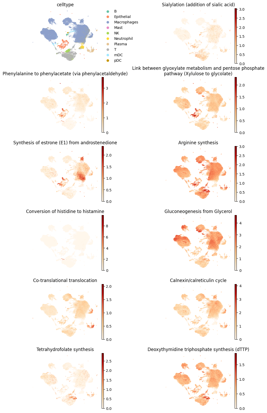
Here we identified a number of metabolic markers, which we can visualize using regular UMAP visualizations.
[16]:
plt.rcParams['figure.figsize'] = (3,3)
plt.rcParams['font.size'] = 10

sc.pl.embedding(results['adata'].metabolic_tasks,
                color=[cell_group] + tf_idf_mrks,
                ncols=2,
                palette=palette,
                frameon=False,
                basis='X_umap',
                wspace=0.7,
                title=["\n".join(textwrap.wrap(t, width=60)) for t in [cell_group] + tf_idf_mrks],
                cmap='OrRd'
               )

We can further inspect the metabolic score distribution across single cells per cell type for these markers.
[17]:
fig, axes = sccellfie.plotting.create_multi_violin_plots(results['adata'].metabolic_tasks,
                                                         features=tf_idf_mrks,
                                                         groupby=cell_group,
                                                         stripplot=False,
                                                         n_cols=3,
                                                         ylabel='Metabolic Score'
                                                        )

Detection using Logistic Regression in Scanpy
Similarly, we can use another approach for identifying metabolic markers. In this case, a logistic regression implemented in Scanpy.
[18]:
method = 'logreg'
sc.tl.rank_genes_groups(results['adata'].metabolic_tasks, cell_group, method=method,
                        use_raw=False, key_added = method)

sc.pl.rank_genes_groups(results['adata'].metabolic_tasks, n_genes=20, sharey=True, key=method, fontsize=4)

[19]:
scanpy_df = sc.get.rank_genes_groups_df(results['adata'].metabolic_tasks,
                                          key=method,
                                          group=None)
In this case we can also inspect them using dot plots.
[20]:
sc.pl.rank_genes_groups_dotplot(results['adata'].metabolic_tasks, n_genes=5, groupby=cell_group,
                                key=method, use_raw=False, standard_scale='var',
                               )
WARNING: dendrogram data not found (using key=dendrogram_celltype). Running `sc.tl.dendrogram` with default parameters. For fine tuning it is recommended to run `sc.tl.dendrogram` independently.

We can further filter the metabolic tasks given the scores assigned by the logistic regression model.
[21]:
scanpy_df['scores'].hist()
[21]:
<Axes: >

[22]:
scores_threshold = 1.0

sc_markers_df = scanpy_df
scanpy_markers = sc_markers_df.loc[sc_markers_df['scores'] > scores_threshold]['names'].unique().tolist()
len(scanpy_markers)
[22]:
11
And perform the same visualizations.
[23]:
plt.rcParams['figure.figsize'] = (3,3)
plt.rcParams['font.size'] = 10

sc.pl.embedding(results['adata'].metabolic_tasks,
                color=[cell_group] + scanpy_markers,
                ncols=2,
                palette=palette,
                frameon=False,
                basis='X_umap',
                wspace=0.7,
                cmap='OrRd',
                title=["\n".join(textwrap.wrap(t, width=60)) for t in [cell_group] + scanpy_markers],
               )
[24]:
fig, axes = sccellfie.plotting.create_multi_violin_plots(results['adata'].metabolic_tasks,
                                                         features=scanpy_markers,
                                                         groupby=cell_group,
                                                         stripplot=False,
                                                         n_cols=3,
                                                         ylabel='Metabolic Score'
                                                        )

Visualize Markers from both methods
We can combine the metabolic tasks from different approaches too:
[25]:
both_markers = sorted(set(tf_idf_mrks + scanpy_markers))
len(both_markers)
[25]:
29
Select only highly active markers
And if we’d like to, we can filter them given their activity level. Here, we first aggregate the metabolic activity of the markers into a cell-type level.
[26]:
agg = sccellfie.expression.aggregation.agg_expression_cells(results['adata'].metabolic_tasks[:, both_markers],
                                                            groupby=cell_group,
                                                            agg_func='trimean')
Then, we filter markers given ther average activity (trimean). Our threshold here was an aggregated score of 1 in at least one cell type.
[27]:
both_markers = agg.T.loc[(agg.T > 1.).any(axis=1)].index.tolist()
len(both_markers)
[27]:
23
And finally, visualize both markers that are “more active”.
[28]:
plt.rcParams['figure.figsize'] = (3,3)
plt.rcParams['font.size'] = 10

sc.pl.embedding(results['adata'].metabolic_tasks,
                color=[cell_group] + both_markers,
                ncols=2,
                palette=palette,
                frameon=False,
                basis='X_umap',
                wspace=0.7,
                cmap='OrRd',
                title=["\n".join(textwrap.wrap(t, width=60)) for t in [cell_group] + both_markers],
               )

[29]:
fig, axes = sccellfie.plotting.create_multi_violin_plots(results['adata'].metabolic_tasks,
                                                         features=both_markers,
                                                         groupby=cell_group,
                                                         stripplot=False,
                                                         n_cols=4,
                                                         ylabel='Metabolic Score'
                                                        )

Differential metabolic analysis
A differential analysis can be done between conditions (per cell type) to identify metabolic changes.
Select conditions to compare
[30]:
adata.obs.condition.unique()
[30]:
['Control', 'Moderate COVID-19', 'Severe COVID-19']
Categories (3, object): ['Control', 'Moderate COVID-19', 'Severe COVID-19']
[31]:
contrasts = [('Control', 'Severe COVID-19')]
condition_key = 'condition'
Perform differential analysis
[32]:
dma = sccellfie.stats.scanpy_differential_analysis(results['adata'].metabolic_tasks,
                                                   cell_type=None,
                                                   cell_type_key=cell_group,
                                                   condition_key=condition_key,
                                                   min_cells=20,
                                                   condition_pairs=contrasts)
Processing DE analysis: 100%|██████████| 10/10 [00:14<00:00, 1.42s/it]
Excluded comparisons due to insufficient cells:

pDC:
  - Control vs Severe COVID-19 (n1=12, n2=76)

Plasma:
  - Control vs Severe COVID-19 (n1=3, n2=1024)

Mast:
  - Control vs Severe COVID-19 (n1=6, n2=39)

Neutrophil:
  - Control vs Severe COVID-19 (n1=0, n2=1603)
Identify significant changes per cell type
After we performed our differential analysis, we need to filter them. We can filter tasks by the adjusted P value (FDR), and by the Cohen’s D, which is a variance-normalized effect size and helps against outliers. If we want to we can further add a threshold for the logFC value, which here we are not doing (logfc_threshold = 0.0).
Typically, a Cohen’s D greater to 0.5 should be a decent effect size. A value of 0.75 should be a good effect size, and if we want to be more strict, we can use a value of 1.0, as done here.
[33]:
cohen_threshold = 1.0
pval_threshold = 0.05
logfc_threshold = 0.0

fig, ax, sig = sccellfie.plotting.create_beeswarm_plot(dma,
                                                       x='cohens_d',
                                                       cohen_threshold=cohen_threshold,
                                                       pval_threshold=pval_threshold,
                                                       logfc_threshold=logfc_threshold,
                                                       show_n_significant=False,
                                                       strip_jitter=True,
                                                       lgd_bbox_to_anchor=(1.01, 1),
                                                       ticks_fontsize=16,
                                                       labels_fontsize=18,
                                                       figsize=(12, 10),
                                                       #save=scCellFie-Diff-Analysis.pdf
                                                      )

[34]:
sig_tasks = sig.reset_index().feature.unique().tolist()
len(sig_tasks)
[34]:
76
Plot number of major task groups up/down regulated
We use our outputs from scCellFie to calculate the number of significant tasks given their major categories located in results['task_info'].
[35]:
sccellfie_db = results
[36]:
def plot_single(condition, ax, pathway, sig_data):
    pathway_counts = {'System': pd.DataFrame(), 'Subsystem': pd.DataFrame()}

    for c, df in sig_data.reset_index().groupby('cell_type'):
        for k, v in pathway_counts.items():
            df2 = df.set_index('feature').join(sccellfie_db['task_info'].set_index('Task'), how='inner')
            df2 = df2.loc[df2.log2FC > 0] if condition == 'up' else df2.loc[df2.log2FC < 0]
            df2 = df2.value_counts(k).to_frame().reset_index()
            df2['cell_type'] = c
            df2 = df2[['cell_type', k, 'count']]
            df2[k] = df2[k].apply(lambda x: x.upper())
            pathway_counts[k] = pd.concat([pathway_counts[k], df2])

    df = pathway_counts[pathway].sort_values('count')
    totals = df.groupby('cell_type')['count'].sum()

    df_normalized = df.copy()
    df_normalized['fraction'] = df.groupby('cell_type')['count'].transform(lambda x: x / x.sum())
    pivoted_data = df_normalized.pivot(index='cell_type', columns=pathway, values='fraction')
    pivoted_data = pivoted_data.sort_index().fillna(0.)

    n_systems = len(pivoted_data.columns)
    colors = glasbey.extend_palette('Set2', palette_size=max([n_systems, 10]))

    pivoted_data.plot(kind='barh', stacked=True, ax=ax, color=colors, legend=False)
    ax.set_xlim((0, 1))
    ax.invert_yaxis()

    ylabels = ax.get_yticklabels()
    ax.tick_params(axis='both', which='major', labelsize=12)

    for idx, cell_type in enumerate(pivoted_data.index):
        ax.text(1.02, idx, f'n={totals[cell_type]:,}', va='center', fontsize=12)

    ax.set_xlabel('Fraction', fontsize=14)
    ax.set_ylabel('')

    return pivoted_data.columns, colors
Then we plot these numbers
[37]:
from matplotlib.colors import to_rgb

pathway = 'System'
condition1_color='#8B0000'
condition2_color='#000080'
fig, (ax1, ax2) = plt.subplots(2, 1, figsize=(3, 6), height_ratios=[1, 1])

legend_elements, colors = plot_single('up', ax1, pathway, sig)
plot_single('down', ax2, pathway, sig)

ax1.set_title('Severe COVID-19', fontsize=16, pad=10, color=to_rgb(condition2_color))
ax2.set_title('Control', fontsize=16, pad=10, color=to_rgb(condition1_color))

plt.figlegend(labels=legend_elements,
              bbox_to_anchor=(0.5, -0.005),
              ncols=2 if pathway == 'System' else 2,
              frameon=False,
              loc='upper center')

plt.subplots_adjust(hspace=0.5)
# For saving this figure, uncomment the code below
# plt.savefig(f'./scCellFie-DA-{pathway}-Combined.pdf',
#             dpi=300,
#             bbox_inches='tight')

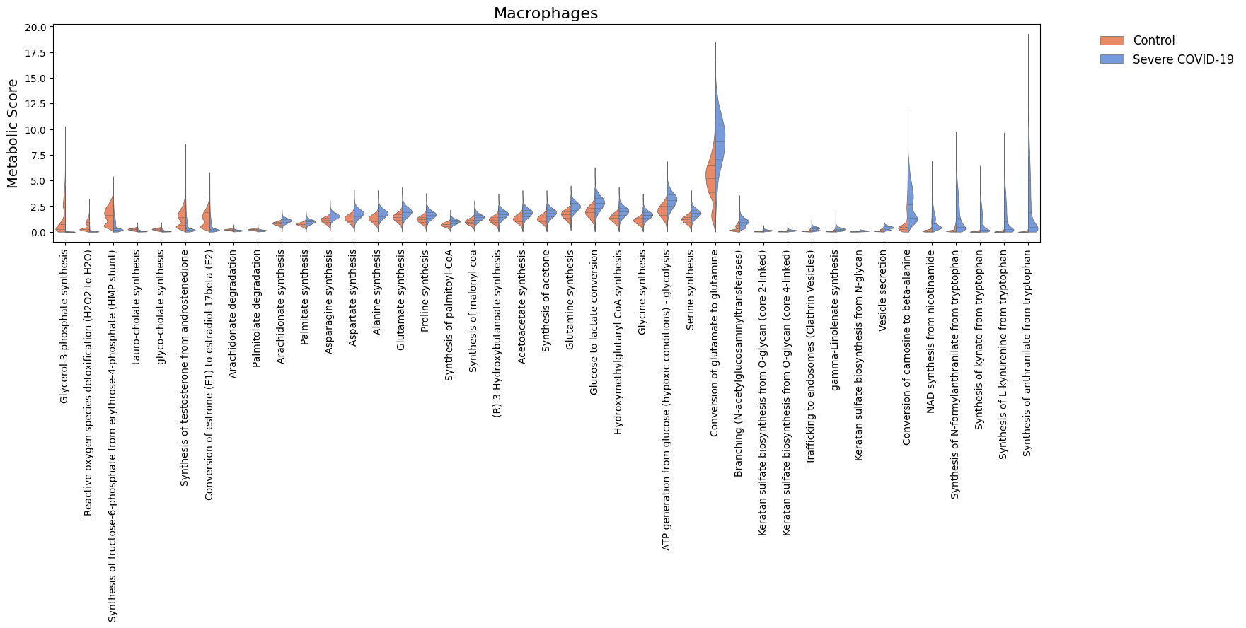
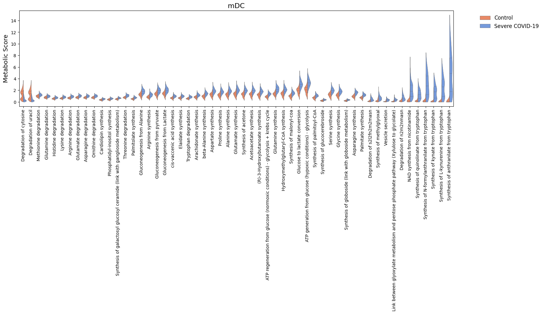
Visualize changes in distributions across single cells
For the significant tasks, we can also compare their distribution of metabolic scores for each condition.
[38]:
cell_show = ['Epithelial', 'Macrophages', 'mDC']

for c in cell_show:
    sig_features = [idx for idx in sig.loc[c].sort_values('log2FC').index]
    N = len(sig_features)
    if N > 0:
        width = min([18, 1.5 + 0.5*N])
        fig, ax = sccellfie.plotting.create_comparative_violin(adata=results['adata'].metabolic_tasks,
                                                               significant_features=sig_features,
                                                               group1='Control',
                                                               group2='Severe COVID-19',
                                                               condition_key=condition_key,
                                                               cell_type_key=cell_group,
                                                               celltype=c,
                                                               xlabel='',
                                                               ylabel='Metabolic Score',
                                                               palette=['coral','cornflowerblue'],
                                                               wrapped_title_length=100,
                                                               figsize=(width, 4),
                                                               fontsize=14,
                                                               title=c,
                                                               tight_layout=False,
                                                               #save=f'DE-Dist-{cname}'
                                                              )

Cell-cell communication
Transfer metabolic tasks into gene expression (all variables in one AnnData object)
Since scCellFie generates separate AnnData objects containing either reaction scores (results['adata'].reactions) or task scores (results['adata'].metabolic_tasks), we need to put both gene expression and metabolic scores into the same AnnData object. Here, we will transfer metabolic scores into the AnnData object containing gene expression.
First, we generate our AnnData with gene expression values in log1p(CP10k).
[39]:
bdata = adata.copy()
Our original adata had raw counts, but after running scCellFie these were converted to CP10k, so we only need to run sc.pp.log1p().
[40]:
sc.pp.log1p(bdata)
We assign a ‘type’ column for the features in each AnnData, so we can easily recognize which are genes and tasks.
[41]:
results['adata'].metabolic_tasks.var['type'] = 'metabolic score'
bdata.var['type'] = 'gene expression'
Now we use a built-in function in scCellFie to transfer features from one source adata into another target adata. In this case we transfer all metabolic tasks (by using var_names=results['adata'].metabolic_tasks.var_names).
[42]:
adata_updated = sccellfie.preprocessing.adata_utils.transfer_variables(
    adata_target=bdata,
    adata_source=results['adata'].metabolic_tasks,
    var_names=results['adata'].metabolic_tasks.var_names
)
[43]:
adata_updated
[43]:
AnnData object with n_obs × n_vars = 63103 × 33755
    obs: 'sample', 'sample_new', 'group', 'disease', 'hasnCoV', 'cluster', 'celltype', 'condition', 'total_counts'
    var: 'type'
    uns: 'normalization', 'neighbors', 'umap', 'log1p'
    obsm: 'X_pca', 'X_umap'
    layers: 'counts'
    obsp: 'distances', 'connectivities'
Compute cell-cell communication based on synthesis and receptor pairs
Using our new AnnData object, we can then compute the communication scores for a list of tuples, where the first element in each tuple is the metabolic task synthesizing the ligand, and the second is its cognate receptor. In this case we use the geometric mean between the cell-type level aggregated values (using the trimean) of metabolic task (ligand) and the log1p(CP10k) gene expression (receptor), for each cell type.
[44]:
ccc_df = sccellfie.communication.compute_communication_scores(adata_updated,
    var_pairs=[('Synthesis of estradiol-17beta (E2) from androstenedione', 'ESR1'), ('Synthesis of L-kynurenine from tryptophan', 'AHR')], # List of LR pairs (synthesis task and receptor)
    groupby=cell_group,
    communication_score='gmean',
    agg_func='trimean',
    ligand_threshold=np.log(2), # Greater than this metabolic activity for consideringing it active
    receptor_threshold=0., # Greater than this expression for considering it active
)
Among the outputs, we get the 'score' columm, containing the geometric mean in this case. Additionlly, this returns the fraction of cells expressing the ligand, and the receptor. These fractions come from the thresholds passed above to say that a metabolic task and a receptor are “active” or “expressed”, respectively.
[45]:
ccc_df
[45]:
| sender_celltype | receiver_celltype | ligand | receptor | score | ligand_fraction | receptor_fraction | |
|---|---|---|---|---|---|---|---|
| 0 | B | B | Synthesis of estradiol-17beta (E2) from andros... | ESR1 | 0.000000 | 0.050505 | 0.000000 |
| 1 | B | B | Synthesis of L-kynurenine from tryptophan | AHR | 0.000000 | 0.095960 | 0.090909 |
| 2 | B | Epithelial | Synthesis of estradiol-17beta (E2) from andros... | ESR1 | 0.000000 | 0.050505 | 0.011173 |
| 3 | B | Epithelial | Synthesis of L-kynurenine from tryptophan | AHR | 0.124446 | 0.095960 | 0.414804 |
| 4 | B | Macrophages | Synthesis of estradiol-17beta (E2) from andros... | ESR1 | 0.000000 | 0.050505 | 0.023146 |
| ... | ... | ... | ... | ... | ... | ... | ... |
| 195 | pDC | T | Synthesis of L-kynurenine from tryptophan | AHR | 0.000000 | 0.141892 | 0.147710 |
| 196 | pDC | mDC | Synthesis of estradiol-17beta (E2) from andros... | ESR1 | 0.000000 | 0.108108 | 0.007439 |
| 197 | pDC | mDC | Synthesis of L-kynurenine from tryptophan | AHR | 0.095979 | 0.141892 | 0.318810 |
| 198 | pDC | pDC | Synthesis of estradiol-17beta (E2) from andros... | ESR1 | 0.000000 | 0.108108 | 0.006757 |
| 199 | pDC | pDC | Synthesis of L-kynurenine from tryptophan | AHR | 0.000000 | 0.141892 | 0.094595 |
200 rows × 7 columns
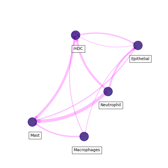
Visualize kynurenine - AHR interactions
In this case we can visualize each of the ligand-receptor interactions we passed. Here, we will visualize the kynurenine synthesis and its AHR receptor interaction.
[46]:
kyn = ccc_df.loc[ccc_df.receptor == 'AHR'].sort_values('score', ascending=False)
For clear visualizations, we can filter important interactions. Below, we first filter by 'score', then by the 'ligand_fraction' and 'receptor_fraction'.
[47]:
### IMPORTANT! THRESHOLD FOR IMPORTANT COMMUNICATION HERE IS MEAN + 1 STD
kyn_thresh = kyn.score.mean() + kyn.score.std()
### AND CELL TYPES EXPRESS LIGAND AND RECEPTOR IN MORE THAN 10% OF CELLS
filtered_kyn = kyn.loc[(kyn.ligand_fraction > 0.1) & (kyn.receptor_fraction > 0.1) & (kyn.score >= kyn_thresh)]
Finally, we can visualize a network of cell types using this ligand-receptor pair.
[48]:
fig, ax = sccellfie.plotting.plot_communication_network(filtered_kyn,
                                                        'sender_celltype',
                                                        'receiver_celltype',
                                                        'score',
                                                        panel_size=(6,6),
                                                        network_layout='spring',
                                                        edge_color='magenta',
                                                        edge_width=8,
                                                        edge_arrow_size=12,
                                                        edge_alpha=0.25,
                                                        node_color='#210070',
                                                        node_size=500,
                                                        node_alpha=0.75,
                                                        node_label_size=10,
                                                        node_label_alpha=0.7,
                                                        node_label_offset=(0.05, -0.2),
                                                        title_fontsize=20,
                                                        tight_layout=True
                                                       )